Latest Posts

• A quick introduction to derivatives for machine learning people

  If you’re like me you probably have used derivatives for a huge part of your life and learned a few rules on how they work and behave without actually understanding where it all comes from. As kids we learn some of these rules early on like the power rule for example in which we know that the derivative of $x^2$ is $2x$ which in a more general form turns to $\frac{dx^a}{dx}=ax^{a-1}$. This is in principle fine since all rules can be readily memorized and looked up in a table. The downside of that is of course that you’re using a system and a formalism that you fundamentally do not understand. Again not necessarily an issue if you are not developing machine learning frameworks yourself on a daily basis but nevertheless it’s really nice to know what’s going on behind the scenes. I myself despise black boxes . So in order to dig a little bit deeper into that I’ll show you what it’s all based on. To do that we have to define what a derivative is supposed to do for you. Do you know? I’m sure you do, but just in case you don’t;

• The importance of context

  When we do modeling it’s of utmost importance that we pay attention to context. Without context there is little that can be inferred.

  Let’s create a correlated dummy dataset that will allow me to highlight my point. In this case we’ll just sample our data from a two dimensional multivariate gaussian distribution specified by the mean vector $\mu_X$ and covariance matrix $\Sigma_X$. We will also create a response variable $y$ which is defined like

  $$y_t\sim N(\mu_{y,t}, \sigma_y)$$ $$\mu_{y,t}=1x_1+1x_2+1x_1 x_2+5$$ $$\sigma_y\sim N(0,20)$$

  where $x_1$ and $x_2$ are realized samples from the two dimensional multivariate guassian distribution above. This covariance matrix looks like this

• Deep Neural Networks in Julia - Love at first sight?

  I love new initiatives that tries to do something fresh and innovative. The relatively new language Julia is one of my favorite languages. It features a lot of good stuff in addition to being targeted towards computational people like me. I won’t bore you with the details of the language itself but suffice it to say that we finally have a general purpose language where you don’t have to compromise expressiveness with efficiency.

• On the apparent success of the maximum likelihood principle

  Today we will run through an important concept in statistical learning theory and modeling in general. It may come as no surprise that my point is as usual “age quod agis”. This is a lifelong strive for me to convey that message to fellow scientists and business people alike. Anyway, back to the topic. We will have a look at why the Bayesian treatment of models is fundamentally important to everyone and not only a select few mathematically inclined experts. The model we will use for this post is a time series model describing Milk sales over time. The model specification is

  $$\begin{align} y_t &\sim N(\mu_t, \sigma)\\ \mu_t &=\sum_{i=1}^{7}\beta_{i} x_{t,i} + \beta_0\\ \sigma &\sim U(0.01, \inf) \end{align}$$

  which is a standard linear model. The $y_t$ is the observed Milk sales units at time $t$ and the $x_{t,i}$ is the indicator variable for weekday $i$ at time $t$. As per usual $\beta_0$ serves as our intercept. A small sample of the data set looks like this

• Building and testing a simple deep learning object detection application

  Deep learning is hot currently. Really hot. The reason for this is that there’s more data available than ever in the space of perception. By perception I mean tasks such as object recognition in images, natural language processing, speech detection etc. Basically anything where we generate copious amounts of data every day. Many companies are putting this data to good use. Google, Facebook, Nvidia, Amazon etc. are all heavy in this space since they have access to most of these data. We as users happily give it to them through all our social media posts and online storage utilization. In any case I wanted to give you all a flavor of what you can do with a relatively small convolutional neural network trained to detect many different objects in an image. Specifically we will use a network architecture known as MobileNet which is meant to run on smaller devices. Luckily for us you can get access to pre-trained models and test it out. So that’s exactly what we’ll do today.

• About identifiability and granularity

  In time series modeling you typically run into issues concerning complexity versus utility. What I mean by that is that there may be questions you need the answer to but are afraid of the model complexity that comes along with it. This fear of complexity is something that relates to identifiability and the curse of dimensionality. Fortunately for us probabilistic programming can handle these things neatly. In this post we’re going to look at a problem where we have a choice between a granular model and an aggregated one. We need to use a proper probabilistic model that we will sample in order to get the posterior information we are looking for.

  The generating model

  In order to do this exercise we need to know what we’re doing and as such we will generate the data we need by simulating a stochastic process. I’m not a big fan of this since simulated data will always be, well simulated, and as such not very realistic. Data in our real world is not random people. This is worth remembering, but as the clients I work with on a daily basis are not inclined to share their precious data, and academic data sets are pointless since they are almost exclusively too nice to represent any real challenge I resort to simulated data. It’s enough to make my point. So without further ado I give you the generating model.

  $$\begin{align} y_t &\sim N(\mu_t, 7)\\ \mu_t &= x_t + 7 z_t\\ x_t &\sim N(3, 1)\\ z_t &\sim N(1, 1) \end{align}$$

  which is basically a gaussian mixture model. So that represents the ground truth. The time series generated looks like this

  

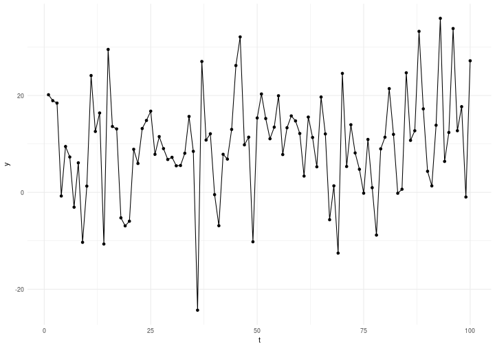
  where time is on the x axis and the response variable on the y axis. The first few lines of the generated data are presented below.

• A gentle introduction to reinforcement learning or what to do when you don't know what to do

  Today we’re going to have a look at an interesting set of learning algorithms which does not require you to know the truth while you learn. As such this is a mix of unsupervised and supervised learning. The supervised part comes from the fact that you look in the rear view mirror after the actions have been taken and then adapt yourself based on how well you did. This is surprisingly powerful as it can learn whatever the knowledge representation allows it to. One caveat though is that it is excruciatingly sloooooow. This naturally stems from the fact that there is no concept of a right solution. Neither when you are making decisions nor when you are evaluating them. All you can say is that “Hey, that wasn’t so bad given what I tried before” but you cannot say that it was the best thing to do. This puts a dampener on the learning rate. The gain is that we can learn just about anything given that we can observe the consequence of our actions in the environment we operate in.

• A few thoughts on apparent bimodality for regression problems!

  Did you ever run into a scenario when your data is showing two distinctive relationships but you’re trying to solve for it with one regression line? This happens to me a lot. So I thought about having some fun with it intead of dreading it and the nasty consequences that may arise from this behaviour. Below you’ll see a plot featuring two variables, $x$, and $y$ where we are tasked with figuring out how the value of $y$ depends on $x$.

• A first look at Edward!

  There’s a new kid on the inference block called “Edward” who is full of potential and promises of merging probabilistic programming, computational graphs and inference! There’s also talk of a 35 times speed up compared to our good old reliable fellow “Stan”. Today I will run some comparisons for problems that currently interest me namely time series with structural hyperparameters.

• On the equivalence of Bayesian priors and Ridge regression

  Today I’m going to take you through the comparison of a Bayesian formalism for regression and compare it to Ridge regression which is a penalized version of OLS. The rationale I have for doing so is that many times in my career I’ve come across “frequentists” who claim that parameters can be controlled via a process called shrinkage, regularization, weight decay, or weight elimination depending on whether you’re using GLM’s, SVM’s or Neural networks. This statement is in principle correct while misguided. The regularization can be seen to arise as a consequence of a probabilistic formulation. I would go so far as to say that there is no such thing as frequentist statistics; there are only those who refuse to add prior information to their model! Before we get started I would like to warn you that this post is going to get a tad mathematical. If that scares you, you might consider skipping the majority of this post and go directly to the summary. Now, let’s go!

  A probabilistic formulation

  Any regression problem can be expressed as an implementation of a probabilistic formulation. For instance what we typically have at our hand is a dependent variable $y$, a matrix $X$ of covariates and a parameter vector $\beta$. The dependent variable consists of data we would like to learn something about or be able to explain. As such we wish to model it’s dynamics via the $\beta$ through $X$. The joint probability distribution for these three ingredients is given simply as $p(y, X, \beta)$. This is the most general form of representing a regression problem probabilistically. However, it’s not very useful, so in order to make it a bit more tangible let’s decompose this joint probability like this.

  $$p(y, X, \beta)=p(\beta\vert y, X)p(y, X)=p(\beta\vert y, X)p(y)p(X)$$

  In this view it is clear that we want to learn something about $\beta$ since that’s the unknowns. The other parts we have observed data on. So we would like to say something clever about $p(\beta\vert y, X)$. How do we go about doing that? Well for starters we need to realize that $p(y, X, \beta)$ can actually be written as

  $$p(y, X, \beta)=p(y\vert \beta, X)p(\beta, X)=p(y\vert \beta, X)p(\beta)p(X)$$

  which means that

  $$p(\beta\vert y, X)p(y)p(X)=p(y\vert \beta, X)p(\beta)p(X)$$

  and therefor

  $$p(\beta\vert y, X)=\frac{p(y\vert \beta, X)p(\beta)}{p(y)}$$

  which is just a derivation of Baye’s rule. Now we actually have something a bit more useful at our hands which is ready to be interpreted and implemented. What do I mean by implemented? Seems like an odd thing to say about probability distributions right? As weird as it may seem we actually haven’t given the probability distributions a concise mathematical representation. This is of course necessary for any kind of inference. So let’s get to it. The first term I would like to describe is the likelihood i.e. the $p(y\vert \beta, X)$ which describes the likelihood of observing the data given the covariance matrix $X$ and a set of parameters $\beta$. For simplicity let’s say this probability distribution is gaussian thus taking the following form $p(y\vert \beta, X)=\mathcal{N}(y-\beta X; 0, \sigma)$. This corresponds to setting up a measurement model $y_t = \beta x_t + \epsilon$ where $\epsilon=\mathcal{N}(0, \sigma)$.

  The second term in the nominator on the right hand side is our prior $p(\beta)$ which we will also consider gaussian. Thus, we will set $p(\beta)=\mathcal{N}(0, \alpha I)$ indicating that the parameters are independant from each other and most likely centered around $0$ with a known standard deviation of $\alpha$. The last term is the denominator $p(y)$ which in this setting functions as the evidence. This is also the normalizing constant that makes sure that we can interpret the right hand side probabilistically.

  That’s it! We now have the pieces we need to push the inference button. This is often for more complicated models done by utilizing Markov Chain Monte Carlo methods to sample the distributions. If we are not interested in the distribution but only the average estimates for the parameters we can just turn this into an optimization problem instead by realizing that

  $$p(\beta\vert y, X)=\frac{p(y\vert \beta, X)p(\beta)}{p(y)}\propto p(y\vert \beta, X)p(\beta)$$

  since $p(y)$ just functions as a normalizing constant and doesn’t change the location of the $\beta$ that would yield the maximum probability. Thus we can set up the optimization problem as

  $$\mathcal{L}(\beta)=\prod_{t=1}^T \mathcal{N}(y_t-\beta x_t; 0, \sigma)\mathcal{N}(\beta; 0, \alpha I)$$

  and maximize this function. Normally when we solve optimization problems it’s easier and nicer to turn it into a minimization problem instead of a maximization problem. This is easily done by minimizing

  $$-\ln \mathcal{L}(\beta)=-\sum_{t=1}^T \ln \mathcal{N}(y_t-\beta x_t; 0, \sigma)- \ln\mathcal{N}(\beta; 0, \alpha I)$$

  as opposed to the equation before. For the sake of clarity let’s assume from now on that we only have one independent variable and only one parameter $\beta$. Since we know that

  $$\mathcal{N}(x;\mu, \sigma)=\frac{1}{\sqrt{2\pi\sigma^2}}\exp\left(-\frac{(x-\mu)^2}{2\sigma^2}\right)$$

  we can easily unfold the logarithms to reveal

  $$-\ln \mathcal{L}(\beta)=-\sum_{t=1}^T\left( -C_1-\frac{\left(y_t-\beta x_t- 0\right)^2}{2\sigma^2}\right) - C_2 + \frac{(\beta-0)^2}{2\alpha^2}$$

  which can be more nicely written as

  $$-\ln \mathcal{L}(\beta)=\sum_{t=1}^T\frac{\left(y_t-\beta x_t\right)^2}{2\sigma^2} + \frac{\beta^2}{2\alpha^2} + C$$

  where $C=TC_1 - C_2$. As such putting a Gaussian prior on your $\beta$ is equivalent penalizing solutions that differ from $0$ by a factor of $1/(2\alpha^2)$ i.e. 1 divided by two times the variance of the Gaussian. Thus, the smaller the variance, the higher our prior confidence is that the solution should be close to zero. The larger the variance the more uncertain we are about where the solution should end up.

  Ridge regression

  The problem of regression can be formulated differently than we did previously, i.e., we don’t need to formulate it probabilistically. In essance what we could do is state that we have a set of independent equations that we would like to solve like this

  $$\Vert X\beta-y\Vert^2$$

  where the variables and parameters have the same interpretation as before. This is basically Ordinary Least Squares (OLS) which suffers from overfitting and sensitivity to outliers and multicollinearity. So what Ridge regression does is to introduce a penalty term to this set of equations like this

  $$\Vert X\beta-y\Vert^2+\Vert \Gamma\beta\Vert^2$$

  where $\Gamma$ is typically chosen to be $\gamma I$. This means that all values in the parameter vector $\beta$ should be close to 0. Continuing along this track we can select a dumbed down version of this equation to show what’s going on for a simple application of one variable $x$ and one parameter $\beta$. In this case

  $$\Vert X\beta-y\Vert^2+\Vert \gamma I\beta\Vert^2$$

  turns into

  $$\sum_{t=1}^T(y_t-\beta x_t)^2+\gamma^2\beta^2$$

  which you may recognize from before. Not convinced? Well let’s look into the differences.

  Probabilistic formulation	Ridge regression
  $\sum_{t=1}^T\frac{\left(y_t-\beta x_t\right)^2}{2\sigma^2} + \frac{\beta^2}{2\alpha^2} + C$	$\sum_{t=1}^T(y_t-\beta x_t)^2+\gamma^2\beta^2$

  Here it’s pretty obvious to see that they are equivalent. The constant $C$ plays no role in the minimization of these expressions. Neither does the denominator $2\sigma^2$. Thus if we set $\lambda=\gamma^2=1/(2\alpha^2)$ the equivalence is clear and we see that what we are really minimizing is

  $$\sum_{t=1}^T(y_t-\beta x_t)^2+\lambda\beta^2$$

  which concludes my point.

  Summary

  So I’ve just shown that ridge regression and a Bayesian formulation with Gaussian priors on the parameters are in fact equivalent mathematically and numerically. One big question remains; Why the hell would anyone in their right mind use a probabilistic formulation for something as simple as penalized OLS? The answer you are looking for here is “freedom”. What if we would have selected a different likelihood? How about a different prior? All of this would have changed and we would have ended up with a different problem. The benefit of the probabilistic approach is that it is agnostic with respect to which distributions you choose. It’s a consistent inferential framework that just allows you the freedom to model things as you see fit. Ridge regression has already made all the model choices for you which is convenient but hardly universal.

  My point is this; whatever model you decide to use and however you wish to model it is your prerogative. Embrace this freedom and don’t let old school convenient tools dictate your way towards solving a specific problem. Be creative, be free and most of all: Be honest to yourself.

  Happy inferencing!

• About choosing your optimization algorithm carefully

  Why is simulation important anyway? Well, first off we need it since many phenomemna (I would even say all interesting phenomemna) cannot be encapsulated by a closed form mathematical expression which is basically what you can do with a pen and paper or a mathematical software. Sounds abstract? Ok, then let me give you an example of why we need simulation. Say you have the job of doing optimization and you have 1 variable where all you have to do is to find a point on the definition range of that variable which gives you the best solution. Let’s say we want to figure the optimal time we need to boil our bolognese for a perfect taste. Now the bolognese can boil from 0 minutes to 1200 minutes which is a very wide range. Say also that we have a way to evaluate whether the bolognese is perfect or not given the amount of minutes it has been cooked. Let’s call this magical evaluation function $f(t)$. Now the annoying thing about $f$ is that we can only evaluate it given a $t$ and we don’t know what it looks like in general. As such we have to search the $t$ for the value that gives the perfect taste.

  

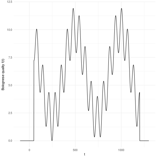
  For this reason we have to search through the entire space, i.e., simulate the function until we have a clear idea of what it looks like. The landscape presented here is just an illustration of what it can look like in a one dimensional problem. Now imagine that you had D dimensions that you cut into M pieces each. You can quickly realize that this space grows exponentially with the number of dimensions $N=M^D$ which is a nasty equation. This basically meanst that if you have 10 variables that you cut into 10 pieces each you will have $10^{10}=10$ billion possible solutions to search through. Does 10 billion sound ok to you? Well, maybe it is. But then let me put in in computing time instead. Let’s say you have a fairly complicated evaluation function such that you can only evaluate $1000$ points per second. This means that you will have to spend $(((10^{10})/1000)/3600)/24\approx 116$ days of simulation time on a computer to search through this landscape. To make matters worse, most variables or parameters you might have to search through rarely decomposes into only 10 valid parts. A more common scenario is that the parameters and variables are continuous by nature which in principle means that the number of “parts” are infinite. For all practical reasons it might mean that you need hundreds of parts for each dimension yielding $((((100^{10})/1000)/3600)/24)/360\approx 3.2$ billion years of computation time. That’s almost as old as our planet which is currently $4.5$ billion years old. We cannot wait that long!

  Luckily most computers today can evaluate more than 200 billion calculations at the same time which means that even our naive calculation comes down to $((((100^{10})/200000000000)/3600)/24)/360\approx 16$ years. This in turn means that if you are able to cut down the number of splits into 40 then you can search through the landscape brute force in $((((40^{10})/200000000000)/3600)) \approx 14.5$ hours. As it turns out science has given us the ability to search through landscapes in a none brute force manner which means that we do not have to evaluate all points that we cut the space into. We can evaluate gradients and also fit functions to data which guides the exploration of the space. This all boils down to that we can in fact search through hundreds of variables and parameters within a day using advanced methods. We will look into some of these methods right now!

  Setting up the experiment

  We would like to optimize the Bolognese quality by tweaking the time we cook it. As we saw above it’s not a nice function to optimize which makes it excellent for hard core testing algorithms for robustness and ability to avoid local maxima.

  Since there are many optimization methods and algorithms I will try to do a benchmark on the most common ones and the ones I like to use. This is not an exhaustive list and there may be many more worthy of adding, but this is the list I know. Hopefully it can guide you in your choices moving forward.

  The algorithms we will look into are primarily implemented in NLopt except the Simulated annealing which comes from the standard optim function in R. Either way the list of algorithms are:

  • Simulated Annealing (SANN)
  • Improved Stochastic Ranking Evolution Strategy (ISRES)
  • Constrained Optimization BY Linear Approximations (COBYLA)
  • Bound Optimization BY Quadratic Approximation (BOBYQA)
  • Low-storage Broyden–Fletcher–Goldfarb–Shanno algorithm (LBFGS)
  • Augmented Lagrangian algorithm (AUGLAG)
  • Nelder-Mead Simplex (NELDERMEAD)
  • Sequential Quadratic Programming (SLSQP)

  As some algorithms (or even most of them) may depend heavily on initial values and starting points we run 500 optimization with randomized starting points for all algorithms. Each algorithm receive the same starting point for each iteration. Thus, each algorithm gets to start it’s optimization in 500 different locations. Seems like a fair setup to me.

  Then let’s get to the results. Below you’ll see a box and whiskers plots of the Optimal Bolognese quality found by each algorithm among the 500 trials. There’s no doubt that all are pretty ok. However, the Augmented lagrangian, Simulated annealing and BFGS are the worst by far. They are also the ones who are the most incosistent. This basically means that they are very sensitive to local maxima and cannot explore the entire landscape properly. This may not be too surprising as they are based on gradient information. Second order or not, it’s still gradient information and that my friends is always local by nature.

  

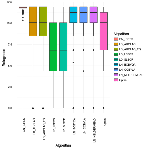
  Where did all the optimizations for the different algorithms go? Let’s make a scatterplot and find out! The continuous line is our original Bolognese function that we want to optimize with respect to the parameter timing $t$.

  

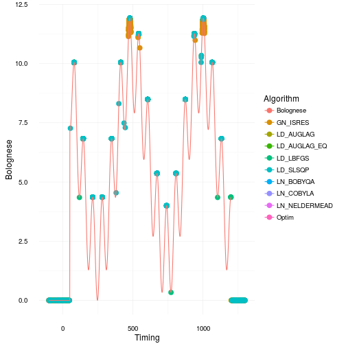
  That looks quite bad actually. Especially for many of the gradient based approaches as they get stuck in local maxima or in regions of 0 gradient. Most of them only find the right solution parts of the time. This is consistent with the box and whiskers plot. However, I would say it’s actually worse than what it appears like in that plot. Just to illustrate how many bad optimization you get have a look at the plot below where we jitter the points across the boxes.

  

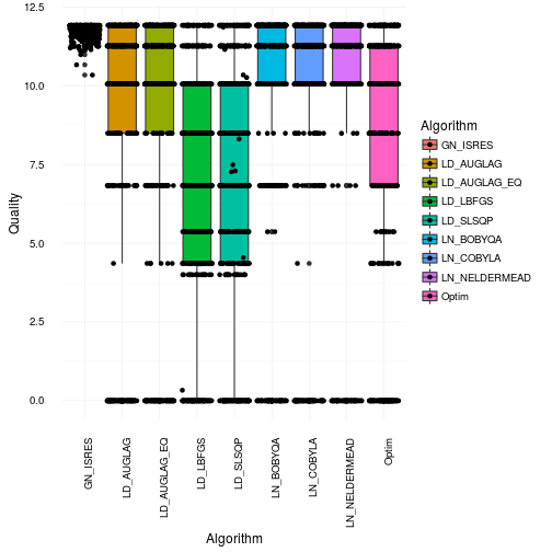
  So where did the optimizations end up on the Bolognese optimization on average? Well in order to see that we will use robust statistics instead to make sure we actually select values that were optmized. Robust statistics in this case will be the median. So now we illustrate the median cook times found by the different algorithms. For fun we will show you the mean results as well. Just for your educational pleasure.

• The truth about priors and overfitting

  Have you ever thought about how strong a prior is compared to observed data? It’s not an entirely easy thing to conceptualize. In order to alleviate this trouble I will take you through some simulation exercises. These are meant as a fruit for thought and not necessarily a recommendation. However, many of the considerations we will run through will be directly applicable to your everyday life of applying Bayesian methods to your specific domain. We will start out by creating some data generated from a known process. The process is the following.

  $$y_t=\sin\left(\frac{x_t}{10}\right)+\cos(z_t)+5d_t+4+\epsilon_t$$

  It features a cyclic process with one event represented by the variable $d$. There is only 1 observation of that event so it means that maximum likelihood will always assign everything to this variable that cannot be explained by other data. This is not always wanted but that’s just life. The data and the maximum likelihood fit looks like below.

• The insignificance of significance

  Statistical significance has always held a slightly magical status in the research community as well as in every other community. This position is unwarrented and the trust that is put in this is severely misguided. If you don’t believe me up front, I understand. So instead of me babbling let’s make a small experiement shall we? Let me ask you the following question:

  Given that the null hypothesis is true; what is the probability of getting a p-value > 0.5?

  Think hard and long on that for a while. ;) Are you done? Good. Here’s the answer: it’s 50 per cent. Wait whaaaaat? Yes, it’s true. The probability of receiving a p-value greater than $0.5$ is 50 per cent. But why? I’ll tell you why!

  The probability distribution of p-values under the null hypothesis is uniform!

  This means that the probability of you getting a p-value of 0.9999 is exactly the same as getting a p-value of 0.0001. This is in principle all fine except for the tiny little piece of annoying practice of interpreting this as a probability of the null hypothesis being true! Nothing could be further from the truth. Interpreting the likelihood of the data as the probability for the hypothesis being true and thus stating

  $$P(D|H_0) = P(H_0|D)$$

  is a logical fallacy.

  No no, you say; surely that cannot be true! Well it is. But don’t let me convince you with math and words. I’d rather show it to you.

  Logical fallacies

  In the wonderful statistical language of R there’s a nice little test called Shapiro-Wilk Normality Test which basically, well uhmm, tests for normality. The null hypothesis $H_0$ in this case is that the samples to test comes from a normal distribution $y\sim N(\mu, \sigma)$. Thus in order to reject the null hypothesis we need a small p-value. For old times sake let’s require this to be less than $0.05$. To start with I will generate 1000 samples from three identical normal distributions with a zero mean and unit variance. They are shown below.

  

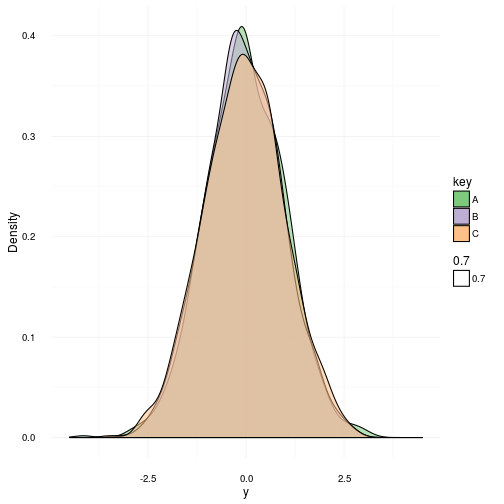
  As you can see they are indeed gaussian distributions and more or less identical. Now I propose an experiment. Let’s do 5000 realized sample sets from the same gaussian distribution featuring 100 samples in each sample set. We will then do the shapiro test on each set and afterwards plot the distribution of all the p-values that came out. Remember: the NULL hypothesis is true in this case since we know all samples come from a $y\sim N(0, 1)$ distribution.

  

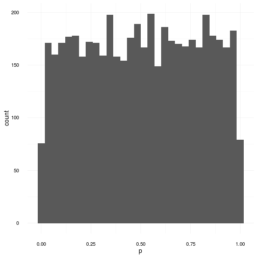
  For the quick minds out there, you can now see that even though we sampled directly from the gaussian distribution and afterwards tried to detect whether it might come from a gaussian or not, we did not get any information. All we got was a “Dude, I really don’t know. It could be anything.” which is of course not very helpful. The reason I have for saying this is again due to the fact that a p-value of 0.001 and a p-value of 0.999 have equal probability under the NULL hypothesis. Thus after these tests we cannot conclude that the generating distribution was gaussian. In fact there is very little we can conclude. We can however say the following:

  We could not successfully refute the NULL hypothesis of the data coming from a gaussian distribution on a 5% significance level.

  but that is also all we can say. This does not make it more probable that the data really comes from a gaussian distribution. Also in this case a p-value of $0.999$ does not make it more probable that it came from a gaussian as compared to a p-value of $0.1$. Now I already hear the opposing people crying “OK, so you’re saying that the statistical tests are useless?”. Well, in fact, that is not what I’m saying. What I’m saying is that they are tricky bastards that must be treated as such. So to back my last statement up let’s look at a scenario where the tests actually do successfully refute something!

  A successful example

  In the following example we repeat the previous experiment but replace the generating distribution with the uniform distribution instead. The resulting p-values are shown in the graph below.

  

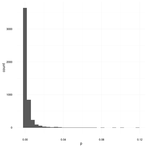
  As you can obviously see the NULL hypothesis in this case is consistently refuted boasting the majority of p-values below $0.05$. This graph here explains the popularity of these tests. In cases where the distributions are obviously not normally distributed the shapiro wilk test and many others successfully declares that it is exceedingly unlikely that this data was generated from a gaussian distribution.

  A talk about hypothesis testing

  Let’s return to the statement of the likelihood vs the probability of the hypothesis being true. I stated

  $$P(D|H_0) \neq P(H_0|D)$$

  But I didn’t say what the relationship really is. To remedy this let’s talk a little about what we really want to achieve with hypothesis testing. In science we are typically looking at binary versions of the hypothesis space where you have a NULL hypothesis $H_0$ and an alternative hypothesis $H_A$ where we would like to evaluate the posterior probability of $H_0$ being true. This is expressed in the following relation.

  $$P(H_0|D) = \frac{P(D|H_0)P(H_0)}{P(D,H_0)+P(D,H_A)} = \frac{1}{1+\frac{P(D,H_A)}{P(D,H_0)}}$$

  This makes it clear that in order to quantify the probability of $H_0$ we have to take the probability of $H_A$ into account. This is not surprising since they are not independant. In fact in order to find the probability of the $H_0$ hypothesis being true given the observed data we need to evaluate the likelihood of the data along with the prior probability of it being true and relating it to the entire evidence for both hypotheses.

  However, we don’t always want to look at hypothesis spaces only featuring two possible outcomes. Actually the fully generalised space of multiple hypotheses looks like this.

  $$P(H_0|D) = \frac{P(D|H_0)P(H_0)}{\sum_i P(D,H_i)}$$

  This relationship is worth remembering each time you design your experiments. It is the foundation of sane science and should not be taken too lightly. This little piece was just to remind you of the dangers of using p-values and plug and play formulas from your statistics classes. So as always here’s a bit of advice

  Write down the model and the assumptions explicitely and then do the inference!

  That’s all for now.

• Implementing predictive sales modeling

  Sales modeling has long been used by clients and media agencies around the world to create insights regarding their historical performance. Most of the efforts have been focused around retrospective projects measuring soft KPI’s, e.g., awareness, liking, penetration etc. In this white paper we’re introducing a new paradigm for implementing a real-time continuous sales modeling setup which can deliver updated learnings and clear-cut recommendations at the time where they’re needed.

• Doing price optimization in R

  As many of us already know R is an extremely useful and powerful language for designing, building and evaluating statistical models. In this example I’m going to use R for calculating the optimal price for a product given very few inputs.

  First off we need to define a simple model for the relationship between sales volume (y) and price change (p).

  $$\ln y = \beta \ln p + a$$

  The variable a is used as a baseline for our sales. Based on this function we can define a profit function that help us calculate the optimal price based on price elasticity, cost per product produced and profit margin. This function is vectorized and is only defined for price elasticities < -1.0 since that is the condition for finding an optimum. For price elasticities > -1.0 we use a heuristic. In any case the closed formula for the optimal price is given by

  $$p=\frac{\beta}{\beta+1}\cdot\frac{c-\lambda}{m}$$

  where $\beta$ is the price elasticity, $c$ the cost of production, $m$ the profit margin and $\lambda$ the penalty term for the case when $\beta >= -1.0$. In this example $\lambda$ is set to 0. Price elasticities greater than -1.0 indicates that if the price increases by 1% then the loss in sales is less than 1%. The R code to implement this function is given below.

• About confidence intervals

  Confidence intervals are as beautiful as they are deceiving. They’re part of an elegant theory of mathematical statistics which has been abused since the dawn of time. Why do I say abused? Well quite frankly because literally everyone gets it wrong.. Now in order to subsantiate my claims let’s have a look at what the confidence interval really is mathematically by inspecting the following formula

  $$P_\theta\left(a(X)<\theta<b(X)\right)=\gamma,\, \forall \theta \in \mathbb{R}$$

  where $X$ is a random sample describing data generated by a process controlled by a fixed parameter $\theta$. The $\gamma$ is the desired confidence level meanwhile the functions $a$ and $b$ are the lower and upper functions generating the boundary of the interval for a random sample. So what does this equation really say? Glad you asked, it states the following:

  For a random sample of the data, the confidence interval as defined by the random variables $a$ and $b$ will contain the true value of the parameter $\theta$ with a probability of $\gamma$.

  An interesting thing about this interval is that it by design has to contain the unknown fixed parameter $\theta$, no matter what that value might be, with a probability of $\gamma$ across all sampled data sets. It does NOT, however, say that the probability that the true value of $\theta$ for a realized data sample lies in the interval calculated for that very sample! Ok, fine! So then why do we state it probabalistically? The answer to this is also simple, because we are stating a probability distribution over random samples of $X$ controlled by the parameter $\theta$. Once we have observed (sampled) a specific realization of that data the probability is gone. The only thing you can state after observing the data, in this setting, is

  The realized interval at hand either contains the true value of the parameter or it does not.

  That’s it folks, there is nothing more you can say about that. Thus, the conclusion here is that confidence intervals only speak about probabilities for repeated samples and measurements of the parameter of interest. In other words, the probability distribution is over the data and not the parameter.

  Now don’t get me wrong, this is a really useful tool to have in your statistical toolbox and will for sure be helpful when you have access to multiple data sets measuring the same phenonemna. However, if you have just one realized data set, then a confidence interval is hardly what you want to express to yourself or others as a finding.

  The remedy