About choosing your optimization algorithm carefully
Why is simulation important anyway? Well, first off we need it since many phenomemna (I would even say all interesting phenomemna) cannot be encapsulated by a closed form mathematical expression which is basically what you can do with a pen and paper or a mathematical software. Sounds abstract? Ok, then let me give you an example of why we need simulation. Say you have the job of doing optimization and you have 1 variable where all you have to do is to find a point on the definition range of that variable which gives you the best solution. Let’s say we want to figure the optimal time we need to boil our bolognese for a perfect taste. Now the bolognese can boil from 0 minutes to 1200 minutes which is a very wide range. Say also that we have a way to evaluate whether the bolognese is perfect or not given the amount of minutes it has been cooked. Let’s call this magical evaluation function . Now the annoying thing about is that we can only evaluate it given a and we don’t know what it looks like in general. As such we have to search the for the value that gives the perfect taste.
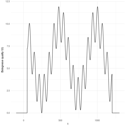
For this reason we have to search through the entire space, i.e., simulate the function until we have a clear idea of what it looks like. The landscape presented here is just an illustration of what it can look like in a one dimensional problem. Now imagine that you had D dimensions that you cut into M pieces each. You can quickly realize that this space grows exponentially with the number of dimensions which is a nasty equation. This basically meanst that if you have 10 variables that you cut into 10 pieces each you will have billion possible solutions to search through. Does 10 billion sound ok to you? Well, maybe it is. But then let me put in in computing time instead. Let’s say you have a fairly complicated evaluation function such that you can only evaluate points per second. This means that you will have to spend days of simulation time on a computer to search through this landscape. To make matters worse, most variables or parameters you might have to search through rarely decomposes into only 10 valid parts. A more common scenario is that the parameters and variables are continuous by nature which in principle means that the number of “parts” are infinite. For all practical reasons it might mean that you need hundreds of parts for each dimension yielding billion years of computation time. That’s almost as old as our planet which is currently billion years old. We cannot wait that long!
Luckily most computers today can evaluate more than 200 billion calculations at the same time which means that even our naive calculation comes down to years. This in turn means that if you are able to cut down the number of splits into 40 then you can search through the landscape brute force in hours. As it turns out science has given us the ability to search through landscapes in a none brute force manner which means that we do not have to evaluate all points that we cut the space into. We can evaluate gradients and also fit functions to data which guides the exploration of the space. This all boils down to that we can in fact search through hundreds of variables and parameters within a day using advanced methods. We will look into some of these methods right now!
Setting up the experiment
We would like to optimize the Bolognese quality by tweaking the time we cook it. As we saw above it’s not a nice function to optimize which makes it excellent for hard core testing algorithms for robustness and ability to avoid local maxima.
Since there are many optimization methods and algorithms I will try to do a benchmark on the most common ones and the ones I like to use. This is not an exhaustive list and there may be many more worthy of adding, but this is the list I know. Hopefully it can guide you in your choices moving forward.
The algorithms we will look into are primarily implemented in NLopt except the Simulated annealing which comes from the standard optim function in R. Either way the list of algorithms are:
- Simulated Annealing (SANN)
- Improved Stochastic Ranking Evolution Strategy (ISRES)
- Constrained Optimization BY Linear Approximations (COBYLA)
- Bound Optimization BY Quadratic Approximation (BOBYQA)
- Low-storage Broyden–Fletcher–Goldfarb–Shanno algorithm (LBFGS)
- Augmented Lagrangian algorithm (AUGLAG)
- Nelder-Mead Simplex (NELDERMEAD)
- Sequential Quadratic Programming (SLSQP)
As some algorithms (or even most of them) may depend heavily on initial values and starting points we run 500 optimization with randomized starting points for all algorithms. Each algorithm receive the same starting point for each iteration. Thus, each algorithm gets to start it’s optimization in 500 different locations. Seems like a fair setup to me.
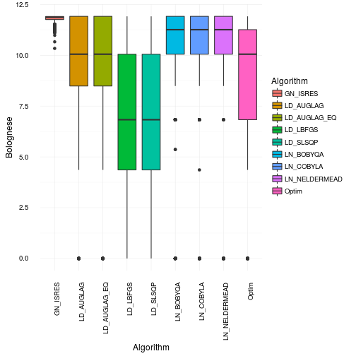
Then let’s get to the results. Below you’ll see a box and whiskers plots of the Optimal Bolognese quality found by each algorithm among the 500 trials. There’s no doubt that all are pretty ok. However, the Augmented lagrangian, Simulated annealing and BFGS are the worst by far. They are also the ones who are the most incosistent. This basically means that they are very sensitive to local maxima and cannot explore the entire landscape properly. This may not be too surprising as they are based on gradient information. Second order or not, it’s still gradient information and that my friends is always local by nature.
Where did all the optimizations for the different algorithms go? Let’s make a scatterplot and find out! The continuous line is our original Bolognese function that we want to optimize with respect to the parameter timing .
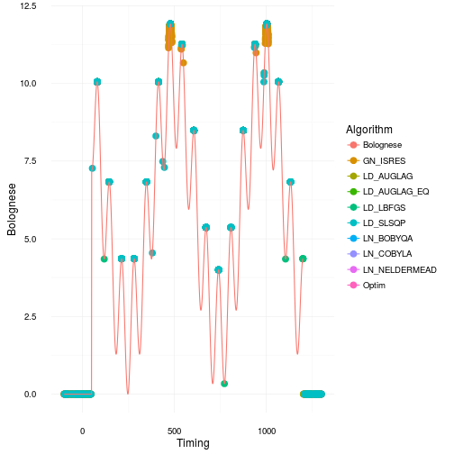
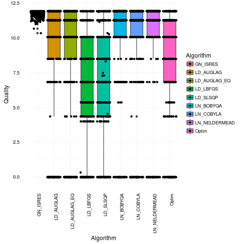
That looks quite bad actually. Especially for many of the gradient based approaches as they get stuck in local maxima or in regions of 0 gradient. Most of them only find the right solution parts of the time. This is consistent with the box and whiskers plot. However, I would say it’s actually worse than what it appears like in that plot. Just to illustrate how many bad optimization you get have a look at the plot below where we jitter the points across the boxes.
So where did the optimizations end up on the Bolognese optimization on average? Well in order to see that we will use robust statistics instead to make sure we actually select values that were optmized. Robust statistics in this case will be the median. So now we illustrate the median cook times found by the different algorithms. For fun we will show you the mean results as well. Just for your educational pleasure.
| Algorithm | Mean | Median | Min | Max |
|---|---|---|---|---|
| GN_ISRES | 11.8 | 11.9 | 10.3 | 11.9 |
| LD_AUGLAG | 8.7 | 10.1 | 0.0 | 11.9 |
| LD_AUGLAG_EQ | 8.8 | 10.1 | 0.0 | 11.9 |
| LD_LBFGS | 6.7 | 6.8 | 0.0 | 11.9 |
| LD_SLSQP | 7.0 | 6.8 | 0.0 | 11.9 |
| LN_BOBYQA | 9.6 | 11.3 | 0.0 | 11.9 |
| LN_COBYLA | 9.4 | 11.3 | 0.0 | 11.9 |
| LN_NELDERMEAD | 10.0 | 11.3 | 0.0 | 11.9 |
| Optim | 8.1 | 10.1 | 0.0 | 11.9 |
The table above is pretty clear. From an optimization point of view the results are clear from both and average, median, worst and best case scenario. The only potential problem here is timing. Evolutionary algorithms are notoriously slow. So experiment with this yourself and see if you get similar results.
Happy inferencing!