A quick introduction to derivatives for machine learning people

If you’re like me you probably have used derivatives for a huge part of your life and learned a few rules on how they work and behave without actually understanding where it all comes from. As kids we learn some of these rules early on like the power rule for example in which we know that the derivative of $x^2$ is $2x$ which in a more general form turns to $\frac{dx^a}{dx}=ax^{a-1}$. This is in principle fine since all rules can be readily memorized and looked up in a table. The downside of that is of course that you’re using a system and a formalism that you fundamentally do not understand. Again not necessarily an issue if you are not developing machine learning frameworks yourself on a daily basis but nevertheless it’s really nice to know what’s going on behind the scenes. I myself despise black boxes . So in order to dig a little bit deeper into that I’ll show you what it’s all based on. To do that we have to define what a derivative is supposed to do for you. Do you know? I’m sure you do, but just in case you don’t;

A derivative is a continuous description of how a function changes with small changes in one or multiple variables.

We’re going to look into many aspects of that statement. For example

• What does small mean?
• What does change mean?
• Why is it continuous?
• How is this useful?

Let’s get to it!

The total and the partial derivative

These terms are typically a source of confusion for many as they are sometimes seen as equivalent and in many cases they seem indistinguishable from one another. They are however not! Let’s start by defining the partial derivative and then move on to the total derivative from there. For this purpose I will use an imaginary function $f\left(t, x, y\right)$ where we have three variables $t$, $x$, and $y$. The partial derivative answers the questions of how $f$ changes ($\partial f$) when one variable changes by a small amount ($\partial x$). In this setting all other variables are assumed to be constant and static. Thus the partial derivative is denoted $\frac{\partial f}{\partial x}$. In order to show what happens when we do this operation we need to first define $f$ as something. Let’s say it looks like this $f(t,x,y)=\frac{4\pi}{3}txy$ which incidentally is the volume of an ellipsoid. Well, perhaps not so incidentally.. Either way I have chosen a different parametrization than is commonly used. In the picture below you can see from top to left to right a sphere, spheroid, and ellipsoid respectively. In our setting we can choose $t=a, x=b, y=c$ for the dimensions.

The partial derivative of the volume of these geometrical spaces then becomes

$$\frac{\partial f}{\partial x}=\frac{4\pi}{3}ty$$

where we have applied the power rule. As you see the $t$ and the $y$ was not touched since we assumed them to be fixed. Thus in the picture above we model what happens with the volume as $b$ extends or shortens by a small amount. This answers our question if they are really independent of $x$. But what if they are not? Well in this case we need the total derivative of $f$ with respect to $x$ which is denoted by $\frac{df}{dx}$ and is defined like this

$$\frac{df}{dx}=\frac{\partial f}{\partial t}\frac{dt}{dx}+\frac{\partial f}{\partial x}\frac{dx}{dx}+\frac{\partial f}{\partial y}\frac{dy}{dx} = \frac{\partial f}{\partial t}\frac{dt}{dx}+\frac{\partial f}{\partial x}+\frac{\partial f}{\partial y}\frac{dy}{dx}$$

where you can see the partial derivative as a part of the total one. So for illustrative purposes let’s constrain the function to a situation where $t=x$. What happens with the derivative then? Well the partial derivative from before stays the same. but the two other terms we need to calculate. The first part becomes $\frac{\partial f}{\partial t}\frac{dt}{dx}=\frac{4\pi}{3}xy \cdot 1$ while the last part turns to $\frac{\partial f}{\partial y}\frac{dy}{dx}=\frac{4\pi}{3}tx \cdot 0=0$. Thus now we get

$$\frac{df}{dx}=\frac{4\pi}{3}xy+\frac{4\pi}{3}ty+0=\frac{4\pi}{3}(t+x)y=\frac{4\pi}{3}2xy$$

by adding the terms and substituting $t=x$ in the last step. Now hopefully it’s apparent that $\frac{\partial f}{\partial x}\neq\frac{df}{dx}$ and that you need to be careful before you state independence between your variables while doing your derivatives.

WAIT! I hear you cry, couldn’t we just do the substitution after we calculated the partial derivative? Indeed you could and you would get something that’s off by a factor 2 which can be substantial. Basically you would get the following insanity

$$\frac{\partial f}{\partial x}=\frac{4\pi}{3}ty=\frac{4\pi}{3}xy\neq \frac{4\pi}{3}2xy$$

This is because what we’re usually after is indeed the total derivative and not the partial. However, you could of course have done the substitution before you calculated the partial derivative. This would turn out nicely like

$$\frac{\partial f}{\partial x}=\frac{\partial }{\partial x} \frac{4\pi}{3}txy=\frac{\partial }{\partial x} \frac{4\pi}{3}x^2y=\frac{4\pi}{3}2xy$$

where we again reach consistency. Thus, you cannot plug in dependencies in your partial derivative after it’s been calculated!

Interpretation as a differential

Let’s return to the definition of the total derivative for a while. Remember that it looked like this

$$\frac{df}{dx} = \frac{\partial f}{\partial t}\frac{dt}{dx}+\frac{\partial f}{\partial x}+\frac{\partial f}{\partial y}\frac{dy}{dx}$$

for a function $f(t,x,y)$ with three variables. Now, if we multiply this by $dx$ everywhere we end up with

$$df = \frac{\partial f}{\partial t}dt+\frac{\partial f}{\partial x}dx+\frac{\partial f}{\partial y}dy$$

which is an expression of a differential view on the function $f$. It states that a very small change in $f$ can be defined like a weighted sum of the small changes in it’s variables where the weights are the partial derivatives of the function with respect to the same variables. We can state this in general for a function $q$ with $M$ variables like this

$$dq=\sum_{i=1}^M\frac{\partial q}{\partial x_i}dx_i$$

which is a much more compact and nice way of looking at it. Writing terms out explicitly quickly becomes tedious. On the flip side of this we also get a compact way of representing our total derivative definition. Again sticking to the function $q$ with it’s $M$ variables.

$$\frac{dq}{dx_p}=\sum_{i=1}^M\frac{\partial q}{\partial x_i}\frac{dx_i}{dx_p}\delta_{ip}+\frac{\partial q}{\partial x_p}$$

The $\delta_{ip}$ is defined to be 1 everywhere except where $i=p$ in which case we define it to $0$. I know that’s not very traditional but it works so I will use the delta function in this way. I do this because

$$\frac{dq}{dx_p}=\sum_{i=1}^M\frac{\partial q}{\partial x_i}\frac{dx_i}{dx_p}$$

while being correct, doesn’t put the focus on the partial derivative of the variable of interest $x_p$ but this is really a matter of taste and not at all important for the usage.

The chain rule of calculus

One of the perhaps most common rules to use when calculating analytical derivatives is the chain rule. Mathematically it basically states the following

$$\frac{df(g(x))}{dx}=\frac{\partial f(g(x))}{\partial g(x)}\frac{dg(x)}{dx}$$

which doesn’t look impressive, but don’t let it’s simplicity fool you. It’s a workhorse without parity in the analytical world of gradients. Remember, $g(x)$ could be anything in this setting. So could $x$ for that matter. As such this rule is applicable to everything relating to gradients.

The chain rule of probability

A small note here regarding naming. The “chain rule” actually exists in probability as well under the name of “The chain rule of probability” or “The general product rule”. I find the latter more natural. In any case that rule states the following

$$p(x,y)=p(x|y)p(y)$$

where $p$ is the probability function for events $x$ and $y$. This rule can be further generalized into $n$ variables by iterating this rule. See the following example:

$$\begin{eqnarray} p(x_1, x_2, x_3, x_4) & = & p(x_1|x_2,x_3,x_4)p(x_2,x_3,x_4) = \\ & = & p(x_1|x_2,x_3,x_4)p(x_2|x_3,x_4)p(x_3,x_4) = \\ & = & p(x_1|x_2,x_3,x_4)p(x_2|x_3,x_4)p(x_3|x_4)p(x_4) \end{eqnarray}$$

You might be forgiven for believing that the order of the variables somehow matter when applying this rule, but of course it doesn’t since all we’re doing is slicing up the probability space into smaller independent patches. So in a more compact format we can express this general rule like this

$$p\left(\bigcap_{k=1}^{n} x_k\right)=\prod_{k=1}^{n}p\left(x_k \bigg| \bigcap_{j=1}^{k-1}x_j\right)$$

where we have used $n$ general variables representing our probability landscape. Now to the reason why i brought this up.

The chain rule of probability has nothing to do with the chain rule of calculus.

So remember to always think of the context if you hear someone name dropping the “chain rule”, since without context it’s quite ambiguous.

Building your own backpropagation engine for deep neural networks

In this section I’ll take you through a simple multi-layered perceptron and a derivation of the backpropagation algorithm. There are many ways to derive this but I’ll start from the error minimization approach which basically describes the fit of a neural network $f(\pmb x, \pmb\theta)$ by the deviance from a known target $y$. The architecture we will solve for is shown in the image below where we have two hidden layers. We stick to this for simplicity. We’ll also only use one output instead of multiple but it’s readily generalizable.

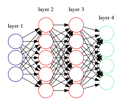
Instead of representing our network graphically we’ll do a more formal representation here where the functional form will be stated mathematically. Basically the functional form will be

$$f(\pmb x_t, \pmb \theta)=\sum_{k=1}^K\tilde\theta_k \left(\varphi\left(\sum_{j=1}^J\hat\theta_{j,k}\varphi\left(\sum_{i=1}^I\theta_{i,j}x_{t,i}\right)\right)\right)$$

where the bold face symbols denotes vectors. The $\varphi(s)=\frac{1}{1+\exp(-a s)}$ function is the sigmoid activation function with a hyperparameter $a$ which we will not tune or care about in this introduction. A small note here, disregarding the $a$ parameter here is really silly since it will fundamentally change the learning of this network. The only reason I allow myself to do it is because it’s beyond the scope to cover it at this point.

In order to train a neural network we need to update the parameters according to how much they affect the error we see. This error can be defined like this for a regression like problem for a data point $(\pmb x_t, y_t)$.

$$E(\pmb x_t,\pmb\theta, y_t)=\frac{1}{2}\left(f(\pmb x_t, \pmb\theta)-y_t\right)^2$$

If we look at the second last layer then we simply update the parameters according to the following rule

$$\hat\theta_{j,k}^{new} = \hat\theta_{j,k}^{old} - \eta\frac{\partial E(\pmb x_t, \pmb\theta, y_t)}{\partial \hat\theta_{j,k}} \forall j,k$$

for each new data point. This is called Stochastic Gradient Descent (SGD). You can read a lot about that in many places so I won’t dive into it here. Suffice it to say that this process can be repeated for each parameter in each layer. So the infamous backpropagation algorithm is just an application of updating your parameters by the partial derivative of the error with respect to that very parameter. Do the partial derivatives for yourself now and see how easy you can derive it. A small trick you can use is to realize that $\varphi '(s)=\varphi(s)(1-\varphi(s))$ where I’ve used the prime notation for a derivative. There’s a nice tutorial on how to do this numerically here.

Take home messages

• The total derivative and the partial derivative are related but at times fundamentally different.
• All constraints and variable substitutions have to be done before calculating the partial derivative.
• The partial derivative ignores implicit dependencies.
• The total derivative takes all dependencies into account.
• Many magic recipes, like the backpropagation algorithm, usually comes from quite simple ideas and doing it for yourself is really instructional and useful.