Did you ever run into a scenario when your data is showing two distinctive relationships but you’re trying to solve for it with one regression line? This happens to me a lot. So I thought about having some fun with it intead of dreading it and the nasty consequences that may arise from this behaviour. Below you’ll see a plot featuring two variables, $x$ , and $y$ where we are tasked with figuring out how the value of $y$ depends on $x$ .

mydf<-tibble(x=seq(0,30,0.2),
             z=ifelse(runif(1:length(x))>0.5, 1, 2),
             y=x*ifelse(z<2, 1, 3)+rnorm(length(x), 0, 5))
ggplot(mydf, aes(y=y, x=x)) + geom_point() + theme_minimal()

plot of chunk problemplot

Naturally, what comes to most peoples mind is that we need to model $y_t=\omega f(x_t)+\epsilon$ where $f$ and $\omega$ are currently unknown. The most straightforward solution to this is to assume that we are in a linear regime and consequently that $f(x)=I(x)=x$ where $I$ is the identity function. The equation then quickly becomes $y_t=\omega x_t+\epsilon$ at which time data scientists usually rejoice and apply linear regression. So let’s do just that shall we.

plot of chunk unnamed-chunk-1

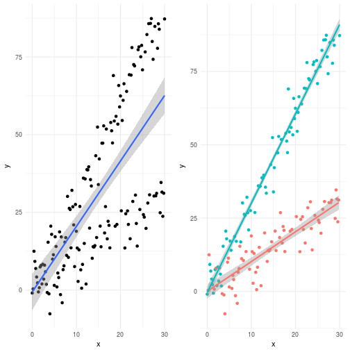
Most of us would agree that the solution with the linear model to the left is not a very nice scenario. We’re always off in terms of knowing the real expectation value. Conceptually this is not very difficult though. We humans do this all the time. If I show you another solution which looks like the one to the right then what would you say? Hopefully you would recognize this as something you would approve of. The problem with this is that a linear model cannot capture this. You need a transformation function to accomplish this.

But wait! We’re all Bayesians here aren’t we? So maybe we can capture this behavior by just letting our model support two modes for the slope parameter? As such we would never really know which slope cluster that would be chosen at any given time and naturally the expectation would end up between the both lines where the posterior probability is zero. Let’s have a look at what the following model does when exposed to this data.

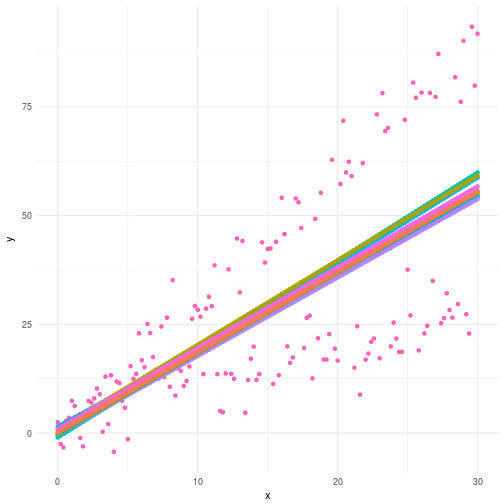
$\begin{align} y_t &\sim \mathcal N(\mu_t, \sigma)\\ \mu_t &=\beta x_t + \alpha\\ \beta &\sim \mathcal C(0, 10)\\ \alpha &\sim \mathcal N(0, 1)\\ \sigma &\sim \mathcal U(0.01, \inf) \end{align}$

Below you can see the plotted simulated regression lines from the model. Not great is it? Not only did our assumption of bimodality fall through but we’re indeed no better of than before. Why? Well, in this case the mathematical formulation of the problem was just plain wrong. Depending on multimodality to cover up for your model specification sins is just bad practice.

plot of chunk prediction plot

Ok, so if the previous model was badly specified then what should we do to fix it? In principle we want the following behavior $y_t=x_t(\beta+\omega z_t)+\alpha$ where $z_t$ is a binary state variable indicating whether the current $x_t$ has the first or the second response type. The full model we then might want to consider looks like this.

$\begin{align} y_t &\sim \mathcal N(\mu_t, \sigma)\\ \mu_t &=x_t(\beta+\omega z_t)+\alpha\\ \omega &\sim \mathcal N(0, 1)\\ z_t &\sim \mathcal{Bin}(1, 0.5)\\ \beta &\sim \mathcal C(0, 10)\\ \alpha &\sim \mathcal N(0, 1)\\ \sigma &\sim \mathcal U(0.01, \inf) \end{align}$

This would allow the state to be modeled as a latent variable in time. This is very useful for a variety of problems where we know something to be true but lack observed data to quantify it. However, modeling discrete latent variables can be computationally demanding if all you are really looking for is an extra dimension. We can of course design this. So instead of viewing $z_t$ as a latent state variable we can actually precode the state by unsupervised hierarchical clustering. The code in R would look like this.

d<-dist(mydf[, c("y", "x")])
hc<-hclust(d)
mydf<-mutate(mydf, zz=cutree(hc, 2))

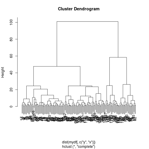
which encodes the clustered state in a variable called $zz$ . Consequently it would produce a hierarchical cluster like the one below.

plot of chunk clusterplot

This leaves us in a position where we can treat $z_t$ as observed data even though we sort of clustered it. The revised math is given below.

$\begin{align} y_t &\sim \mathcal N(\mu_t, \sigma)\\ \mu_t &=x_t(\beta+\omega z_t)+\alpha\\ \omega &\sim \mathcal N(0, 1)\\ \beta &\sim \mathcal C(0, 10)\\ \alpha &\sim \mathcal N(0, 1)\\ \sigma &\sim \mathcal U(0.01, \inf) \end{align}$

Comparing the results from our first model with the current one we can see that we’re obviously doing better. The clustering works pretty well. The graph to the left is the first model and the one to the right is the revised model with an updated likelihood.

plot of chunk 1vs2

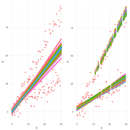
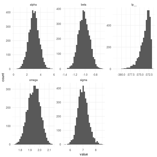
As is always instructional let’s look at the posteriors of the parameters of our second model. They are depicted below. You can clearly see that the “increase in slope” parameter $\omega$ clearly captures the new behavior we wished to model.

plot of chunk model results

Conclusion

This post has been about not becoming blind with respect to the mathematical restrictions we impose on the total model by sticking to a too simplistic representation. Also in this case the Bayesian formalism does not save us with it’s bimodal capabilities since the model was misspecified.

Think about all aspects of your model before you push the inference button
Be aware that something that might appear as a clear cut case for multimodality may actually be a pathological problem in your model
Also, be aware that sometimes multimodality is expected and totally ok

Happy inferencing!