Today we will run through an important concept in statistical learning theory and modeling in general. It may come as no surprise that my point is as usual “age quod agis”. This is a lifelong strive for me to convey that message to fellow scientists and business people alike. Anyway, back to the topic. We will have a look at why the Bayesian treatment of models is fundamentally important to everyone and not only a select few mathematically inclined experts. The model we will use for this post is a time series model describing Milk sales over time. The model specification is

$\begin{align} y_t &\sim N(\mu_t, \sigma)\\ \mu_t &=\sum_{i=1}^{7}\beta_{i} x_{t,i} + \beta_0\\ \sigma &\sim U(0.01, \inf) \end{align}$

which is a standard linear model. The $y_t$ is the observed Milk sales units at time $t$ and the $x_{t,i}$ is the indicator variable for weekday $i$ at time $t$ . As per usual $\beta_0$ serves as our intercept. A small sample of the data set looks like this

y	WDay1	WDay3	WDay4	WDay5	WDay6	WDay7
4331	0	1	0	0	0	0
6348	0	0	1	0	0	0
5804	0	0	0	1	0	0
6897	0	0	0	0	1	0
8428	0	0	0	0	0	1
6725	1	0	0	0	0	0

which, for the response variable $y$ , looks like the distributional plot below.

plot of chunk problemplot

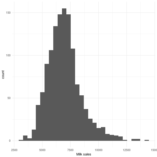
For those of you wth modeling experience you will see that a mere intra-weekly seasonality will not be enough for capturing all the interesting parts of this particular series but for the point I’m trying to make it will work just fine sticking with seasonality + and intercept.

Estimating the parameters of the model

We’re going to estimate the parameters of this model by

The full Bayesian treatment, i.e., we’re going to estimate $p(\beta\vert y, X)$
The Maximum likelihood, i.e., we’re going to estimate $p(y\vert \beta, X)$ which in the tables and the plots will be referred to as “Freq” from the term “Frequentist” which I inherently dislike but I made the tables and plots a while ago so bear with me.

If you rememeber your probability theory training you know that $p(\beta\vert y, X) \neq p(y\vert \beta, X)$ . Sure but so what? Well, this matters a lot. In order to see why let’s dig into these terms. First off, let’s have a look at the proper full Bayesian treatment. We can express that posterior distribution using three terms, namely the

Likelihood,
the Prior and
the Evidence.

$p(\beta\vert y, X)=\frac{p(y\vert \beta, X)p(\beta\vert X)}{\int p(y,\beta, X) d\beta}$

The Evidence is the denominator and serves as a normalization factor that allows us to talk about probabilities in the first place. The nominator consists of two terms; the Likelihood (to the left), and the prior (to the right). It’s worth noticing here that the prior for $\beta$ may very well depend on the covariates as such, and even on the response variable should we wish to venture into emperical priors. Explained in plain words the equation above states that we wish to estimate the posterior probability of our parameters $\beta$ by weigting our prior knowledge and assumptions about those parameters with the plausability of them generating a data set like ours, normalized by the plausability of the data itself under the existing mathematical model. Now doesn’t that sound reasonable? I think it does.

Now if we look into the same kind of analysis for what the Maximum Likelihood method does we find the following equation

$p(y\vert \beta, X)=\frac{p(\beta\vert y, X)}{p(\beta\vert X)}\int p(y,\beta, X) d\beta$

which states that the probability of observing a data set like ours given fixed $\beta$ ’s is the posterior probability of the $\beta$ ’s divided by our prior assumptions scaled by the total plausability of the data itself. Now this also sounds reasonable, and it is. The only problem is that the quantity on the left hand side is not sampled; it is maximized in Maximum Likelihood. Hence the name.. On top of that what you do in 99% of all cases is ignore the right hand side in the equation above and just postulate that $p(y\vert \beta,X)=\mathcal{N}(\mu,\sigma)$ which is a rather rough statement to begin with, but let’s not dive into that right now. So when you maximize this expression, what are you actually doing? Tadam! You’re doing data fitting. This might seem like a good thing but it’s not. Basically you’re generating every conceivable hypothesis known to the model at hand and picking the one that happens to coincide the best with your, in most cases, tiny dataset. That’s not even the worst part; The worst part is that you won’t even, once the fitting is done, be able to express yourself about the uncertainty of the parameters of your model!

Now that we have skimmed through the surface of the math behind the two methodologies we’re ready to look at some results and do the real analysis.

Technical setup

The Bayesian approach is estimated using the probabalistic programming language Stan following the model described in the beginning, i.e., we have completely uninformed priors. This is to make it as similar to the Maximum Likelihood method as possible. The Maximum Likelihood method is implemented using the lm function in R. Thus, in R we’re simply doing

mylm <- lm(y~WDay1+WDay2+WDay3+WDay4+WDay5+WDay6+WDay7, data=ourdata)

meanwhile in Stan we’re doing the following, admittedly a bit more complicated, code.

data {
  int< lower = 0 > N;       // Number of data points
  vector[N] y;              // The response variable
  matrix[N, 7] xweekday;    // The weekdays variables
}
 
parameters {
  real b0;  // The intercept
  vector[7] bweekday;       // The weekday regression parameters
  real< lower = 0 > sigma;  // The standard deviation
}
 
transformed parameters {
  vector[N] mu;                // Declaration
  mu = b0 + xweekday*bweekday; // The mean prediction each timestep
}
 
model {
  y ~ normal(mu, sigma);    // Likelihood
}
 
generated quantities {
  vector[N] yhat;
  yhat = b0 + xweekday * bweekdayhat;
}

If you’re not in the mood to learn Stan you can achieve the same thing by using the brms package in R and run the following code

require(brms)
mybrms <- brm(bf(y~WDay1+WDay2+WDay3+WDay4+WDay5+WDay6+WDay7), data=ourdata, cores = 2, chains = 4)

which will write, compile and sample your model in Stan and return it to R.

Results

Now to the dirty details of our calculations for the parameter estimates of the model. Throughout the results we will discuss the Bayesian estimation first and then the ML-approach. This pertains to each plot and or table. The first result we will have a look at is the estimates themselves. For the Bayesian estimates we have the average values and the uncertainty expresses as an estimation error. For the ML approach we have the estimates and a standard error. Have a look.

	Estimate	Est.Error	Estimate	Std. Error
Intercept	75539	450271	8866	83
WDay1	-67911	450271	-1231	117
WDay2	-68249	450270	-1571	117
WDay3	-68560	450269	-1882	117
WDay4	-69072	450270	-2396	117
WDay5	-69754	450270	-3076	117
WDay6	-69723	450270	-3045	117
WDay7	-66678	450270	NA	NA

If you’re looking at the table above, you might think “What the damn hell!?”, Bayesian statistics makes no sense at all! Why did we get these crazy estimates? Look at the nice narrow confidence intervals on the right hand side of the table generated by the maximum likelihood estimates and compare them to the wide credibility intervals to the left. You might be forgiven for dismissing the results from the Bayesian approach, since the difference is quite subtle from a mathematical point of view. After all we are computing the exact same mathematical model. The difference is our reasoning about the parameters. If you remember correctly maximum likelihood views the parameters as fixed constants without any variation. The variation you see in maximum likelihood comes from the uncertainty about the data and not the parameters! This is important to remember. The “Std. Error” from the maximum likelihood estimate has nothing to do with uncertainty about the parameter values for the observed data set. Instead it’s uncertainty regarding what would happen to the estimates if we observed more data sets that looks like ours. Remember from the section above that, Statistically speaking, what ML does is maximize $p(y\vert \beta,X)$ which expresses likelihood over different $y$ ’s given an observed and fixed set of parameters $\beta$ along with covariates $X$ .

But ok, maybe you think there’s something very fishy with this model since the estimates are so different. How could we possible end up capturing the same time series? Well, rest assured that we can. Below you can see a scatter plot between the Observed response $y$ and the predicted $\hat{y}$ for the Bayesian and ML estimation. Pretty similar huh? We can also have a look at the average fitted values from the Bayesian estimation and the fitted values from the ML method. As you can see they agree to an rather high degree.

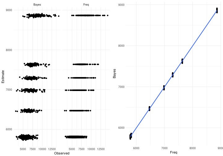
Plot over the agreement between the fitting of the two approaches. The lefthand side shows the fitted vs observed for the Bayesian and the ML. The right hand side shows a scatterplot of the fitted from both approaches.

Graphs can be quite decieving though so let’s do our homework and quantify how good these models really are head to head.

Model validation and sanity checking

I’ll start by taking you through the standard measures of goodness within time series analysis. Specifically we have the following measures.

Mean Absolute Error (MAE)
Mean Absolute Standard Error (MASE)
Mean Absolute Percentage Error (MAPE)
Root Mean Square Error (RMSE)
Normalized Root Mean Square Error (NRMSE)
Coefficient of Variation Root Mean Square Error (CVRMSE)
Proportion of variance explained (R²)

These are quantified in the table below and as you can see there’s virtually no difference between the two estimations. The reason for this is of course that they were built with the same open assumptions about which values that are plausible. In fact both estimation procedures almost accept anything that’s consistent with the data at hand.

	Bayes	Freq
MAE	803.19	803.63
MASE	0.79	0.79
MAPE	0.12	0.12
RMSE	1117.51	1117.01
NRMSE	0.10	0.10
CVRMSE	0.16	0.16
R2	0.45	0.45

So again it seems like there’s not much differentiating these models from one another. That is true while looking at the result of the average fitted values from the two estimates. However, there’s a massive difference in the interpretation of the model. What do I mean by that you might ask yourself, and it’s a good question because if the fit is apparently more or less the same we should be able to pick any of the methods right? Wrong! Remember what I said about sampling being important as it unveils structure in the parameter space that is otherwise hidden through the ML approach. In the illustration below you can see the posterior density of each $\beta$ for the weekday effects. Here it’s clear that they can take many different values which ends up in equally good models. This is the reason why our uncertainty is huge in the Bayesian estimation. There is really a lot of probable parameter values that could be assumed by the model. Also present in the illustration is the ML estimate indicated by a dark vertical line.

plot of chunk posteriorsbeta

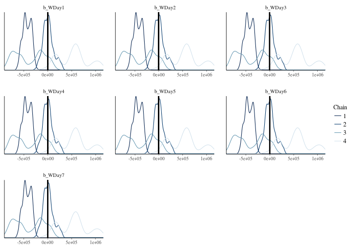
If you look closely there are at least two or three major peaks in the densities which denotes the highest probability for those parameters (In this plot we have four different MCMC chains for each parameter), so why on earth is ML so crazy sure about the parameter values? If you read my post you already know the answer, as we already discussed that the error/uncertainty expressed by the ML approach has nothing to do with the uncertainty of the parameters. It’s purely an uncertainty about the data. As such there is no probabilistic interpretation of the parameters under the ML methodology. They are considered as fixed constants. It’s the data that’s considered to be random.

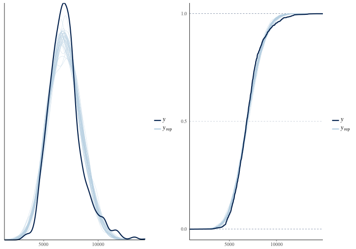
There is one more important check that we need to do and that’s a posterior predictive check just to make sure that we are not biased too much in our estimation. Again inspecting the density and cumulative distribution function below we can see that we’re doing quite ok given that we only have day of week as covariates in our model.

plot of chunk posteriorpredict

Diving into the intercept

As you saw previously there’s way more support for different values of our parameters than the ML method shows us. To further visualize this we’ll take a look at the samples for the intercept $\beta_0$ chain by chain using violin plots. They show the distribution on the y axis and the chain id on the x axis. As before the ML estimate is indicated by a black horizontal line. You can see that the ML approach only agrees with the expected value of chain number 2. The other support is completely ignored and not exposed to the user.

plot of chunk interceptviolin

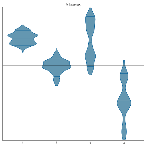
Why is this an issue one might wonder, and the answer to that is that there is no guarantee that chain number two is the one that best represents the physical reality we’re trying to model. The purpose of any model is (or at least should be) to understand the underlying physical reality that we’re interested in. As such the company selling the Milk that we just modeled might ask how much is my Base sales each day? We know that we can answer this because that is what we’re capturing using the intercept in our model. Let’s answer these questions based on our estimations

Mrs. Manager: “So Miss Data Scientist, what’s our base sales?”

Miss Data Scientist: “Well I have two answers for you. I will answer it using two uninformed approaches; an ML approach and a Bayesian approach. Here goes.”

Bayesian answer: Your base sales is 75,539 which never happens and depending on the day is reduced by around -68,563.8 yielding an average Saturday sales of 8,861.
Maximum likelihood answer: Your base sales is 8,866 which happens on an average Saturday. All other days this is reduced by an average of -2,200

The summaries you can see in this table.

Weekday	AvgSalesBayes	AvgSalesFreq
Sun	7,628	7,635
Mon	7,289	7,295
Tue	6,979	6,984
Wed	6,466	6,470
Thu	5,785	5,790
Fri	5,816	5,821
Sat	8,861	8,866

Mrs. Manager: “That doesn’t make sense to me at all. Just pick the best performing model”

Miss Data Scientist: “They’re both equally good performance wise.”

Mrs. Manager: “I don’t like this at all!”

Miss Data Scientist: “Me too.”

What you should do

So now that we have established that the Bayesian approach is necessary and useful the question still remains on how to fix the estimation. We will do two things to improve upon the estimation

Set up informed priors for our believs about the plausability of the parameters
Save the sampler some time by setting a baseline for the weekdays

Basically we will modify the model like this

$\begin{align} y_t &\sim N(\mu_t, \sigma)\\ \mu_t &=\sum_{i=1}^{7}\beta_{i} x_{t,i} + \beta_0\\ \beta_0 &\sim N(\mu_y^{emp}, \sigma_y^{emp})\\ \beta_i &\sim N(0, \sigma_y^{emp}) \forall i\in[1,7]\\ \sigma &\sim U(0.01, \infty) \end{align}$

where $\mu_y^{emp}$ and $\sigma_y^{emp}$ are the empirical mean and standard deviation of the response variable respectively. This is a nice practical hack since it makes sure that your priors are in the vicinity of the response you’re trying to model. The resulting code is given below. You can try it on your own daily time series. It’s quite plug and play.

data {
  int< lower = 0 > N;       // Number of data points
  vector[N] y;          // The response variable
  matrix[N, 7] xweekday; // The weekdays variables
}
 
parameters {
  real< lower = 0.01 > b0;  // The intercept
  vector[7 - 1] bweekday; // The weekday regression parameters
  real< lower = 0 > sigma;  // The standard deviation
}
 
transformed parameters {
  // Declarations
  vector[N] mu;
  vector[7] bweekdayhat;
 
  // The weekday part
  bweekdayhat[1] = 0;
  for (i in 1:(7 - 1) ) bweekdayhat[i + 1] = bweekday[i];
  
  // The mean prediction each timestep
  mu = b0 + xweekday*bweekdayhat;
}
 
model {
  // Priors
  b0 ~ normal(mean(y), sd(y));
  bweekday ~ normal(0, sd(y));
 
  // Likelihood
  y ~ normal(mu, sigma);
}
 
generated quantities {
  vector[N] yhat;
  yhat = b0 + xweekday * bweekdayhat;
}

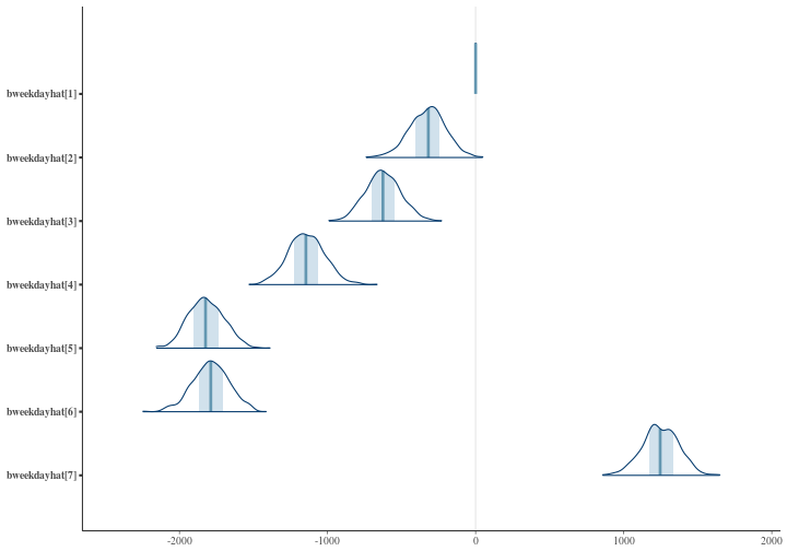
Now let’s have a look at this model instead. A quick look into these parameters show that we have nice clean unimodal posteriors due to our prior beliefs being applied to the analysis. The same table as shown previously is not shown below with the results for the new estimation appended to the rightmost side. For clarification we name the columns Estimate and SD.

	Estimate	Est.Error	Estimate	Std. Error	Estimate	SD
Intercept	75,539	450,271	8,866	83	7,615	89
WDay1	-67,911	450,271	-1,231	117	0	0
WDay2	-68,249	450,270	-1,571	117	-324	122
WDay3	-68,560	450,269	-1,882	117	-624	118
WDay4	-69,072	450,270	-2,396	117	-1,141	123
WDay5	-69,754	450,270	-3,076	117	-1,819	119
WDay6	-69,723	450,270	-3,045	117	-1,788	124
WDay7	-66,678	450,270	NA	NA	1,249	122

As you can see these estimates are quite different and to the naked eye makes more sense from what we know about the data set and what we can expect from intra-weekly effects. We can further check these estimates by inspecting the posteriors further. Note here the “bweekdayhat[1]” which is a delta distribution at 0. This serves as our baseline for the intra-week effect that we’re capturing. The x-axis in the plot are the estimated $\beta_i$ ’s and the y-axis for each parameter is the posterior probability density.

plot of chunk intervalplots

So from a model estimation standpoint we should be pretty happy now. But how does this new estimation compare to the others? Below I will repeat the model performance table from earlier and extend it with our new “Bayes2” estimation.

	Bayes	Freq	Bayes2
MAE	803.19	803.63	803.21
MASE	0.79	0.79	0.79
MAPE	0.12	0.12	0.12
RMSE	1117.51	1117.01	1117.05
NRMSE	0.10	0.10	0.10
CVRMSE	0.16	0.16	0.16
R2	0.45	0.45	0.45

It’s evident that our new way of estimating the parameters of the model yields not only a more satisfying modeling approach but also provides us with a more actionable model without any reduction from a performance perspective. I’d call that a win win. Basically this means that our data scientist can go back with confidence and approach the manager again with robust findings and a knowledge about the space of potentially plausible parameters!

Summary and finishing remarks

Today we looked at how to use Bayesian analysis applied to a real world problem. We saw the dangers in applying the maximum likelihood method blindly. Moreover we saw that the Bayesian formalism forces you to make your assumptions explicit. If you don’t it will show you all possibilities that the mathematical models supprts given the data set. This is important to remember and it is NOT a problem with the Bayesian analysis; It is a feature! So if I can leave you with some recommendations and guidelines when dealing with models I would say this:

There’s nothing wrong in experimenting with ML methods for speady development of prototype models but whenever you are going to quantify your trust in your model you have to and I mean have to sample it and treat it in a proper probabilistic, i.e., Bayesian formalism.
Always make your assumptions and beliefs explicit in your final model. This will help not only you but fellow modelers who might use your model moving forward.
Learn to understand the difference between Maximum Likelihood and Sampling the posterior probability distribution of your parameters. It might be hard at first but it will be worth it in the end.
Accept that there is no such thing as an analysis without assumptions! When you’re doing linear regression using Maximum Likelihood you are effectively assuming that any value between minus infinity and plus infinity are equally likely and that is nonsense my friend.

Happy inferencing!