About identifiability and granularity

In time series modeling you typically run into issues concerning complexity versus utility. What I mean by that is that there may be questions you need the answer to but are afraid of the model complexity that comes along with it. This fear of complexity is something that relates to identifiability and the curse of dimensionality. Fortunately for us probabilistic programming can handle these things neatly. In this post we’re going to look at a problem where we have a choice between a granular model and an aggregated one. We need to use a proper probabilistic model that we will sample in order to get the posterior information we are looking for.

The generating model

In order to do this exercise we need to know what we’re doing and as such we will generate the data we need by simulating a stochastic process. I’m not a big fan of this since simulated data will always be, well simulated, and as such not very realistic. Data in our real world is not random people. This is worth remembering, but as the clients I work with on a daily basis are not inclined to share their precious data, and academic data sets are pointless since they are almost exclusively too nice to represent any real challenge I resort to simulated data. It’s enough to make my point. So without further ado I give you the generating model.

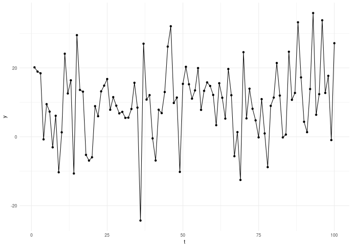
$\begin{align} y_t &\sim N(\mu_t, 7)\\ \mu_t &= x_t + 7 z_t\\ x_t &\sim N(3, 1)\\ z_t &\sim N(1, 1) \end{align}$

which is basically a gaussian mixture model. So that represents the ground truth. The time series generated looks like this

plot of chunk problemplot12

where time is on the x axis and the response variable on the y axis. The first few lines of the generated data are presented below.

t	y	x	z
0	20.411003	2.314330	1.0381077
1	22.174020	2.512780	1.5292838
2	-5.035160	2.048367	-0.1099282
3	1.580412	1.627389	1.2106257
4	-5.391217	4.924959	-0.4488093
5	-1.360732	3.237641	-0.1645335

So it’s apparent that we have three variables in this data set; the response variable $y$ , and the covariates $x$ and $z$ ( $t$ is just an indicator of a fake time). So the real model is just a linear model of the two variables. Now say that instead we want to go about solving this problem and we have two individuals arguing about the best solution. Let’s call them Mr. Granularity and Mr. Aggregation. Now Mr. Granularity is a fickle bastard as he always wants to split things into more fine grained buckets. Mr. Aggregation on the other hand is more kissable by nature. By that I’m refering to the Occam’s razor version of kissable, meaning “Keep It Simple Sir” (KISS).

This means that Mr. Granularity wants to estimate a parameter for each of the two variables while Mr. Aggregation wants to estimate one parameter for the sum of $x$ and $z$ .

Mr. Granularity’s solution

So let’s start out with the more complex solution. Mathematically Mr. Granularity defines the probabilistic model like this

$\begin{align} y_t &\sim N(\mu_t, \sigma)\\ \mu_t &=\beta_x x_t + \beta_z z_t + \beta_0\\ \beta_x &\sim N(0, 5)\\ \beta_z &\sim N(0, 5)\\ \beta_0 &\sim N(0, 5)\\ \sigma &\sim U(0.01, \inf) \end{align}$

which is implemented in Stan code below. There’s nothing funky or noteworthy going on here. Just a simple linear model.

data {
  int N;
  real x[N];
  real z[N];
  real y[N];
}
parameters {
  real b0;
  real bx;
  real bz;
  real<lower=0> sigma;
}
model {
  b0 ~ normal(0, 5);
  bx ~ normal(0, 5);
  bz ~ normal(0, 5);
  for(n in 1:N)
    y[n] ~ normal(bx*x[n]+bz*z[n]+b0, sigma);
}
generated quantities {
  real y_pred[N];
  for (n in 1:N)
    y_pred[n] = x[n]*bx+z[n]*bz+b0;
}

Mr. Aggregation’s solution

So remember that Mr. Aggregation was concerned about over-fitting and didn’t want to split things up into the most granular pieces. As such, in his solution, we will add the two variables $x$ and $z$ together and quantify them as if they were one. The resulting model is given below followed by the implementation in Stan.

$\begin{align} y_t &\sim N(\mu_t, \sigma)\\ \mu_t &=\beta_r (x_t + z_t) + \beta_0\\ \beta_r &\sim N(0, 5)\\ \beta_0 &\sim N(0, 5)\\ \sigma &\sim U(0.01, \inf) \end{align}$

data {
  int N;
  real x[N];
  real z[N];
  real y[N];
}
parameters {
  real b0;
  real br;
  real<lower=0> sigma;
}
model {
  b0 ~ normal(0, 5);
  br ~ normal(0, 5);
  for(n in 1:N)
    y[n] ~ normal(br*(x[n]+z[n])+b0, sigma);
}
generated quantities {
  real y_pred[N];
  for (n in 1:N)
    y_pred[n] = (x[n]+z[n])*br+b0;
}

Analysis

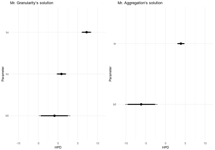
Now let’s have a look at the different solutions and what we end up with. This problem was intentionally noise to confuse even the granular approach as much as possible. We’ll start by inspecting the posteriors for the parameters of interest. They’re shown below in these caterpillar plots where the parameters are on the y-axis and the posterior density is given on the x-axis.

plot of chunk distributions

It is clear that the only direct comparison we can make is the intercept $b_0$ from both models. Now if you remember, the generating function doesn’t contain an intercept. It’s $0$ . Visually inspecting the graphs above will show you that something bad is happening to both models. Let’s put some numbers on this shall we. The Tables below will illuminate the situation.

Parameter distributions - Granular model

	mean	2.5%	25%	50%	75%	97.5%
b0	-0.88	-4.86	-2.21	-0.89	0.49	3.14
bx	0.88	-0.41	0.44	0.87	1.32	2.15
bz	7.21	5.89	6.77	7.23	7.66	8.49

Mr. Granularity have indeed identified a possible intercept with the current model. The mean value of the posterior is -0.88 and as you can see there is 33% probability mass larger than $0$ indicating the models confidence that there is an intercept. The model expresses the same certainty about the fact that $\beta_x$ and $\beta_z$ are real given that 91% and 100% of their masses respectively are above $0$ . The absolute errors for the models estimate are -0.12 and 0.21 for $\beta_x$ and $\beta_z$ respectively.

Parameter distributions - Aggregated model

	mean	2.5%	25%	50%	75%	97.5%
b0	-6.11	-10.19	-7.47	-6.14	-4.77	-1.99
br	3.89	2.90	3.56	3.89	4.22	4.89

Mr. Aggregation have also identified a possible intercept with the current model. The mean value of the posterior is -6.11 and as you can see there is 0% probability mass larger than $0$ indicating the models confidence that there is an intercept. The model expresses the same certainty about the fact that $\beta_r$ is real given that 100% of it’s mass is above $0$ . The absolute errors for the models estimate are 2.89 and -3.11 if you consider the distance from the true $\beta_x$ and $\beta_z$ respectively.

Comparing the solutions

The table below quantifies the differences between the estimated parameters and the parameters of the generating function. The top row are the true parameter values from the generating function and the row names are the different estimated parameters in Mr. A’s and Mr. G’s model respectively.

	b0	bx	bz
Mr. A b0	6.11
Mr. A br		2.89	3.11
Mr. G b0	0.88
Mr. G bx		0.12
Mr. G bz			0.21

As is apparent from the table you can see that Mr. Aggregation’s model is 289% off with respect to the true $\beta_x$ coefficient, and 44% off with respect to the true $\beta_z$ coefficient. That’s not very impressive and actually leads to the wrong conclusions when trying to discern the dynamics of $x$ and $z$ on $y$ .

The corresponding analysis for the granular model gives us better results. Mr. Granularity’s model is 12% off with respect to the true $\beta_x$ coefficient, and 3% off with respect to the true $\beta_z$ coefficient. This seems a lot better. But still, if we have a granular model, why are we so off on the intercept? Well if you remember the generating function from before it looked like this

$\begin{align} y_t &\sim N(\mu_t, 7)\\ \mu_t &= x_t + 7 z_t\\ x_t &\sim N(3, 1)\\ z_t &\sim N(1, 1) \end{align}$

which is statistically equivalent with the follwoing formulation

$\begin{align} y_t &\sim N(\mu_t, 7)\\ \mu_t &= x_t + 7 z_t + 3\\ x_t &\sim N(0, 1)\\ z_t &\sim N(1, 1)\\ \end{align}$

which in turn would make the $x_t$ variable nothing but noise. This can indeed be confirmed if you simulate many times. This is one of the core problems behind some models; identifiability. It’s a tough thing and the very reason why maximum likelihood can not be used in general. You need to sample!

Conclusion

I’ve shown you today the dangers of aggregating information into a single unit and what those dangers are. There is a version of the strategy shown here which brings the best of both worlds; Hierarchical pooling. This methodology pulls data with low information content towards the mean of the other more highly informative ones. The degree of pooling can be readily expressed as a prior belief on how much the different subparts should be connected. As such; don’t throw information away. If you believe they belong together, express that belief as a prior. Don’t restrict your model to the same biases as you have! In summary:

Always add all the granularity you need to solve the problem
Don’t be afraid of complexity; it’s part of life
Always sample the posteriors when you have complex models
Embrace the uncertainty that your model shows
Be aware that the uncertainty quantified is the model’s uncertainty

Happy Inferencing!