The importance of context

When we do modeling it’s of utmost importance that we pay attention to context. Without context there is little that can be inferred.

Let’s create a correlated dummy dataset that will allow me to highlight my point. In this case we’ll just sample our data from a two dimensional multivariate gaussian distribution specified by the mean vector $\mu_X$ and covariance matrix $\Sigma_X$ . We will also create a response variable $y$ which is defined like

$y_t\sim N(\mu_{y,t}, \sigma_y)$ $\mu_{y,t}=1x_1+1x_2+1x_1 x_2+5$ $\sigma_y\sim N(0,20)$

where $x_1$ and $x_2$ are realized samples from the two dimensional multivariate guassian distribution above. This covariance matrix looks like this

	X1	X2
X1	3.0	2.5
X2	2.5	3.0

where the correlation between our variables are obvious. So let’s plot each variable against it’s response and have a look. As you can see it’s quite apparent that the variables are rather similar.

Sigma <- matrix(c(3, 2.5, 2.5, 3), 2, 2)
mydf <- as_tibble(data.frame(mvrnorm(500, c(10, 10), Sigma))) %>% 
    mutate(y = 1 * X1 + 1 * X2 + 1 * X1 * X2 + 5 + rnorm(length(X1), 0, 20))
gather(mydf, variable, value, -y) %>% 
    ggplot(aes(y = y, x = value, color = variable)) +
    geom_point() + geom_smooth() + xlab("Variable value") + ylab("y") + 
    facet_grid(. ~ variable)

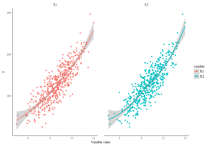
plot of chunk dataplotforvariables

What would you expect us to get from it if we fit a simple model? We have generated 500 observations and we are estimating 4 coefficients. Should be fine right? Well it turns out it’s not fine at all. Not fine at all. Remember that we defined our coefficients to be 1 both for the independent effects and for the interaction effects between $x_1$ and $x_2$ . The intercept is set to $5$ . In other words we actually have point parameters here behind the physical model. This is an assumption that in most modeling situations would be crazy, but we use it here to highlight a point. Let’s make a linear regression model with the interaction effects present.

mylm <- lm(y~X1+X2+X1:X2, data=mydf)

In R you specify interaction effects like this “:” which might look a bit weird but just accept it for now. It could have been written in other ways but I like to be explicit. Now that we have this model we can investigate what it says about our unknown parameters that we estimated.

	y
	B	CI	std. Error	p
(Intercept)	14.88	-27.29 – 57.05	21.46	.489
X1	0.06	-4.56 – 4.68	2.35	.981
X2	0.13	-4.47 – 4.74	2.34	.955
X1:X2	1.09	0.66 – 1.52	0.22	<.001
Observations	500
R² / adj. R²	.783 / .781

A quick look at the table reveals a number of pathologies. If we look at the intercept we can see that it’s 198 per cent off. For the $x_1$ and $x_2$ variables we’re -94 and -87 per cent off respectively. The interaction effect ends up being 9 percent off target which is not much. All in all though, we’re significantly off the target. This is not surprising though. In fact, I would have been surprised had we succeeded. So what’s the problem? Well, the problem is that our basic assumption of independence between variables quite frankly does not hold. The reason why it doesn’t hold is because the generated data is indeed correlated. Remember our covariance matrix in the two dimensional multivariate gaussian.

Let’s try to fix our analysis. In this setting we need to introduce context and the easiest most natural way to deal with that are priors. To do this we cannot use our old trusted friend “lm” in R but must resort to a bayesian framework. Stan makes that very simple. This implementation of our model is not very elegant but it will neatly show you how easily you can define models in this language. We simply specify our data, parameters and model. We set the priors in the model part. Notice here that we don’t put priors on everything. For instance. I might know that a value around 1 is reasonable for our main and interaction effects but I have no idea of where the intercept should be. In this case I will simple be completely ignorant and not inject my knowledge into the model about the intercept because I fundamentally believe I don’t have any. That’s why $\beta_0$ does not appear in the model section.

data {
  int<lower=0> N;
  real y[N];
  real x1[N];
  real x2[N];
}
parameters {
  real b0;
  real b1;
  real b2;
  real b3;
  real<lower=1> sigma;
}
model {
  b1 ~ normal(1, 0.5);
  b2 ~ normal(1, 0.5);
  b3 ~ normal(1, 0.5);
  for(i in 1:N) y[i] ~ normal(b0+b1*x1[i]+b2*x2[i]+b3*x1[i]*x2[i], sigma);
}

If we go ahead and run this model we get the inference after the MCMC engine is done. The summary of the bayesian model can be seen below where the coefficients make a lot more sense.

##                mean         sd          2.5%        97.5%
## b0        6.2015899 4.50797603 -2.399446e+00    15.161352
## b1        0.9823694 0.48849017  5.569159e-02     1.949283
## b2        0.9775408 0.47906798  6.376570e-02     1.912414
## b3        1.0014422 0.04332279  9.151089e-01     1.084912
## sigma    20.0924148 0.62945656  1.890865e+01    21.342656
## lp__  -1747.7225224 1.64308492 -1.751779e+03 -1745.557799

If we look at the distributions for our parameters we can see that in the right context we capture the essense of our model but moreover we also see the support the data gives to the different possible values. We select 80 percent intervals here to illustrate the width of the distribution and the mass.

plot of chunk histogramsex1

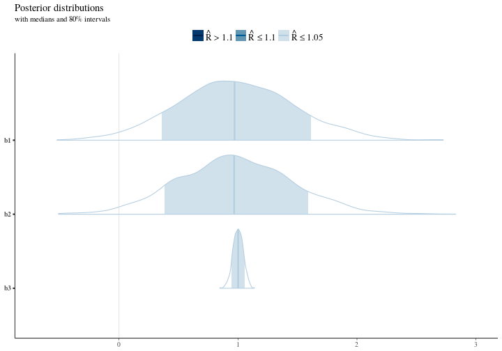
Notice here that we are around the right area and we don’t get the crazy results that we got from our regression earlier. This is because of our knowledge (context) of the problem. The model armed with our knowledge correctly realizes that there are many possible values for the intercept and the width of that distribution is a testement to that. Further there’s some uncertainty about the value for the main effects in the model meanwhile the interaction effect is really nailed down and our estimate here is not uncertain at all.