The insignificance of significance

Statistical significance has always held a slightly magical status in the research community as well as in every other community. This position is unwarrented and the trust that is put in this is severely misguided. If you don’t believe me up front, I understand. So instead of me babbling let’s make a small experiement shall we? Let me ask you the following question:

Given that the null hypothesis is true; what is the probability of getting a p-value > 0.5?

Think hard and long on that for a while. ;) Are you done? Good. Here’s the answer: it’s 50 per cent. Wait whaaaaat? Yes, it’s true. The probability of receiving a p-value greater than $0.5$ is 50 per cent. But why? I’ll tell you why!

The probability distribution of p-values under the null hypothesis is uniform!

This means that the probability of you getting a p-value of 0.9999 is exactly the same as getting a p-value of 0.0001. This is in principle all fine except for the tiny little piece of annoying practice of interpreting this as a probability of the null hypothesis being true! Nothing could be further from the truth. Interpreting the likelihood of the data as the probability for the hypothesis being true and thus stating

$$P(D|H_0) = P(H_0|D)$$

is a logical fallacy.

No no, you say; surely that cannot be true! Well it is. But don’t let me convince you with math and words. I’d rather show it to you.

Logical fallacies

In the wonderful statistical language of R there’s a nice little test called Shapiro-Wilk Normality Test which basically, well uhmm, tests for normality. The null hypothesis $H_0$ in this case is that the samples to test comes from a normal distribution $y\sim N(\mu, \sigma)$. Thus in order to reject the null hypothesis we need a small p-value. For old times sake let’s require this to be less than $0.05$. To start with I will generate 1000 samples from three identical normal distributions with a zero mean and unit variance. They are shown below.

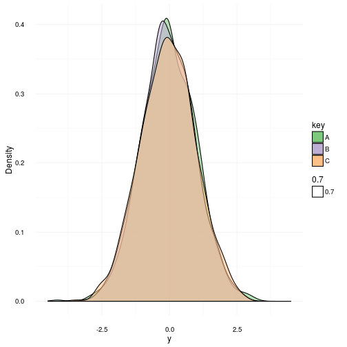
As you can see they are indeed gaussian distributions and more or less identical. Now I propose an experiment. Let’s do 5000 realized sample sets from the same gaussian distribution featuring 100 samples in each sample set. We will then do the shapiro test on each set and afterwards plot the distribution of all the p-values that came out. Remember: the NULL hypothesis is true in this case since we know all samples come from a $y\sim N(0, 1)$ distribution.

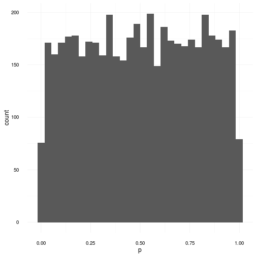
For the quick minds out there, you can now see that even though we sampled directly from the gaussian distribution and afterwards tried to detect whether it might come from a gaussian or not, we did not get any information. All we got was a “Dude, I really don’t know. It could be anything.” which is of course not very helpful. The reason I have for saying this is again due to the fact that a p-value of 0.001 and a p-value of 0.999 have equal probability under the NULL hypothesis. Thus after these tests we cannot conclude that the generating distribution was gaussian. In fact there is very little we can conclude. We can however say the following:

We could not successfully refute the NULL hypothesis of the data coming from a gaussian distribution on a 5% significance level.

but that is also all we can say. This does not make it more probable that the data really comes from a gaussian distribution. Also in this case a p-value of $0.999$ does not make it more probable that it came from a gaussian as compared to a p-value of $0.1$. Now I already hear the opposing people crying “OK, so you’re saying that the statistical tests are useless?”. Well, in fact, that is not what I’m saying. What I’m saying is that they are tricky bastards that must be treated as such. So to back my last statement up let’s look at a scenario where the tests actually do successfully refute something!

A successful example

In the following example we repeat the previous experiment but replace the generating distribution with the uniform distribution instead. The resulting p-values are shown in the graph below.

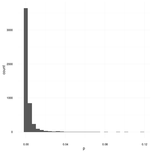
As you can obviously see the NULL hypothesis in this case is consistently refuted boasting the majority of p-values below $0.05$. This graph here explains the popularity of these tests. In cases where the distributions are obviously not normally distributed the shapiro wilk test and many others successfully declares that it is exceedingly unlikely that this data was generated from a gaussian distribution.

A talk about hypothesis testing

Let’s return to the statement of the likelihood vs the probability of the hypothesis being true. I stated

$$P(D|H_0) \neq P(H_0|D)$$

But I didn’t say what the relationship really is. To remedy this let’s talk a little about what we really want to achieve with hypothesis testing. In science we are typically looking at binary versions of the hypothesis space where you have a NULL hypothesis $H_0$ and an alternative hypothesis $H_A$ where we would like to evaluate the posterior probability of $H_0$ being true. This is expressed in the following relation.

$$P(H_0|D) = \frac{P(D|H_0)P(H_0)}{P(D,H_0)+P(D,H_A)} = \frac{1}{1+\frac{P(D,H_A)}{P(D,H_0)}}$$

This makes it clear that in order to quantify the probability of $H_0$ we have to take the probability of $H_A$ into account. This is not surprising since they are not independant. In fact in order to find the probability of the $H_0$ hypothesis being true given the observed data we need to evaluate the likelihood of the data along with the prior probability of it being true and relating it to the entire evidence for both hypotheses.

However, we don’t always want to look at hypothesis spaces only featuring two possible outcomes. Actually the fully generalised space of multiple hypotheses looks like this.

$$P(H_0|D) = \frac{P(D|H_0)P(H_0)}{\sum_i P(D,H_i)}$$

This relationship is worth remembering each time you design your experiments. It is the foundation of sane science and should not be taken too lightly. This little piece was just to remind you of the dangers of using p-values and plug and play formulas from your statistics classes. So as always here’s a bit of advice

Write down the model and the assumptions explicitely and then do the inference!

That’s all for now.