A gentle introduction to reinforcement learning or what to do when you don't know what to do
Today we’re going to have a look at an interesting set of learning algorithms which does not require you to know the truth while you learn. As such this is a mix of unsupervised and supervised learning. The supervised part comes from the fact that you look in the rear view mirror after the actions have been taken and then adapt yourself based on how well you did. This is surprisingly powerful as it can learn whatever the knowledge representation allows it to. One caveat though is that it is excruciatingly sloooooow. This naturally stems from the fact that there is no concept of a right solution. Neither when you are making decisions nor when you are evaluating them. All you can say is that “Hey, that wasn’t so bad given what I tried before” but you cannot say that it was the best thing to do. This puts a dampener on the learning rate. The gain is that we can learn just about anything given that we can observe the consequence of our actions in the environment we operate in.
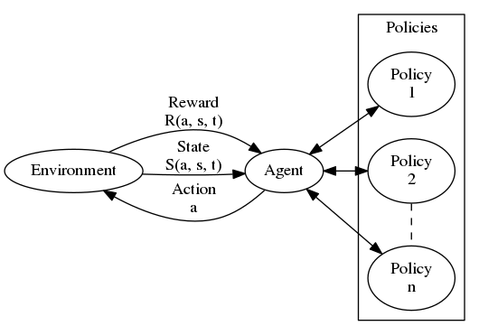
As illustrated above, reinforcement learning can be thought of as an agent acting in an environment and receiving rewards as a consequence of those actions. This is in principle a Markov Decision Process (MDP) which basically captures just about anything you might want to learn in an environment. Formally the MDP consists of
- A set of states
- A set of actions
- A set of rewards
- A set of transition probabilities
which looks surprisingly simple but is really all we need. The mission is to learn the best transition probabilities that maximizes the expected total future reward. Thus to move on we need to introduce a little mathematical notation. First off we need a reward function which gives us the reward that comes from taking action in state at time . We also need a transition function which will give us the next state . The actions are generated by the agent by following one or several policies. A policy function therefore generates an action which will, to it’s knowledge, give the maximum reward in the future.
The problem we will solve - Cart Pole
We will utilize an environment from the OpenAI Gym called the Cart pole problem. The task is basically learning how to balance a pole by controlling a cart. The environment gives us a new state every time we act in it. This state consists of four observables corresponding to position and movements. This problem has been illustrated before by Arthur Juliani using TensorFlow. Before showing you the implementation we’ll have a look at how a trained agent performs below.
As you can see it performs quite well and actually manages to balance the pole by controlling the cart in real time. You might think that hey that sounds easy I’ll just generate random actions and it should cancel out. Well, put your mind at ease. Below you can see an illustration of that approach failing.
So to the problem at hand. How can we model this? We need to make an agent that learns a policy that maximizes the future reward right? Right, so at any given time our policy can choose one of two possible actions namely
- move left
- move right
which should sound familiar to you if you’ve done any modeling before. This is basically a Bernoulli model where the probability distribution looks like this . Once we know this the task is to model as a function of the current state . This can be done by doing a linear model wrapped by a sigmoid like this
where are the four parameters that will basically control which way we want to move. These four parameters makes up the policy. With these two pieces we can set up a likelihood function that can drive our learning.
where is defined above. This likelihood we want to maximize and in order to do that we will turn it around and instead minimize the negative log likelihood
which can be solved for our simple model by setting
and doing the math. However, we want to make this general enough to support more complex policies. As such we will employ gradient descent updates to our parameters .
where is the learning rate. This can also be considered to change over time dynamically but for now let’s keep it plain old vanilla. This is it for the theory. Now let’s get to the implementation!
Implementation
As the AI Gym is mostly available in Python we’ve chosen to go with that language. This is by no means my preferred language for data science, and I could give you 10 solid arguments as to why it shouldn’t be yours either, but since this post is about machine learning and not data science I won’t expand my thoughts on that. In any case, Python is great for machine learning which is what we are looking at today. So let’s go ahead and import the libraries in Python3 that we’re going to need.
import numpy as np
import math
import gym
After this let’s look at initiating our environment and setting some variables and placeholders we are going to need.
env = gym.make('CartPole-v0')

# Configuration
state = env.reset()
max_episodes = 2000
batch_size = 5
learning_rate = 1
episodes = 0
reward_sum = 0
params = np.random.normal([0,0,0,0], [1,1,1,1])
render = False

# Define place holders for the problem
p, action, reward, dreward = 0, 0, 0, 0
ys, ps, actions, rewards, drewards, gradients = [],[],[],[],[],[]
states = state
Other than this we’re going to use some functions that needs to be defined. I’m sure multiple machine learning frameworks have implemented it already but it’s pretty easy to do and quite instructional so why not just do it. ;)
The python functions you’re going to need
As we’re implementing this in Python3 and it’s not always straightforward what is Python3 and Python2 I’m sharing the function definitions with you that I created since they are indeed compliant with the Python3 libraries. Especially Numpy which is an integral part of computation in Python. Most of these functions are easily implemented and understood. Make sure you read through them and grasp what they’re all about.
def discount_rewards(r, gamma=1-0.99):
    df = np.zeros_like(r)
    for t in range(len(r)):
        df[t] = np.npv(gamma, r[t:len(r)])
    return df

def sigmoid(x):
    return 1.0/(1.0+np.exp(-x))

def dsigmoid(x):
    a=sigmoid(x)
    return a*(1-a)

def decide(b, x):
    return sigmoid(np.vdot(b, x))

def loglikelihood(y, p):
    return y*np.log(p)+(1-y)*np.log(1-p)

def weighted_loglikelihood(y, p, dr):
    return (y*np.log(p)+(1-y)*np.log(1-p))*dr

def loss(y, p, dr):
	return -weighted_loglikelihood(y, p, dr)

def dloss(y, p, dr, x):
    return np.reshape(dr*( (1-np.array(y))*p - y*(1-np.array(p))), [len(y),1])*x
Armed with these function we’re ready to do the main learning loop which is where the logic of the agent and the training takes place. This will be the heaviest part to run through so take your time.
The learning loop
while episodes < max_episodes:
    if reward_sum > 190 or render==True:
        env.render()
        render = True
    p = decide(params, state)
    action = 1 if p > np.random.uniform() else 0
    state, reward, done, _ = env.step(action)
    reward_sum += reward
    # Add to place holders
    ps.append(p)
    actions.append(action)
    ys.append(action)
    rewards.append(reward)
    # Check if the episode is over and calculate gradients
    if done:
        episodes += 1
        drewards = discount_rewards2(rewards)
        drewards -= np.mean(drewards)
        drewards /= np.std(drewards)
        if len(gradients)==0:
            gradients = dloss(ys, ps, drewards, states).mean(axis=0)
        else:
            gradients = np.vstack((gradients, dloss(ys, ps, drewards, states).mean(axis=0)))
        if episodes % batch_size == 0:
            params = params - learning_rate*gradients.mean(axis=0)
            gradients = []
            print("Average reward for episode", reward_sum/batch_size)
            if reward_sum/batch_size >= 200:
                print("Problem solved!")
            reward_sum = 0
        # Reset all
        state = env.reset()
        y, p, action, reward, dreward, g = 0, 0, 0, 0, 0, 0
        ys, ps, actions, rewards, drewards = [],[],[],[],[]
        states = state
    else:
        states=np.vstack((states, state))

env.close()
Phew! There it was, and it wasn’t so bad was it? We now have a fully working reinforcement learning agent that learns the CartPole problem by policy gradient learning. Now, for those of you who know me you know I’m always preaching about considering all possible solutions that are consistent with your data. So maybe there are more than one solution to the CartPole problem? Indeed there is. The next section will show you a distribution of these solutions across the four parameters.
Multiple solutions
So we have solved the CartPole problem using our learning agent and if you run it multiple times you will see that it converges to different solutions. We can create a distribution over all of these different solutions which will inform us about the solution space of all possible models supported by our parameterization. The plot is given below where the x axis are the parameter values and the y axis the probability density.
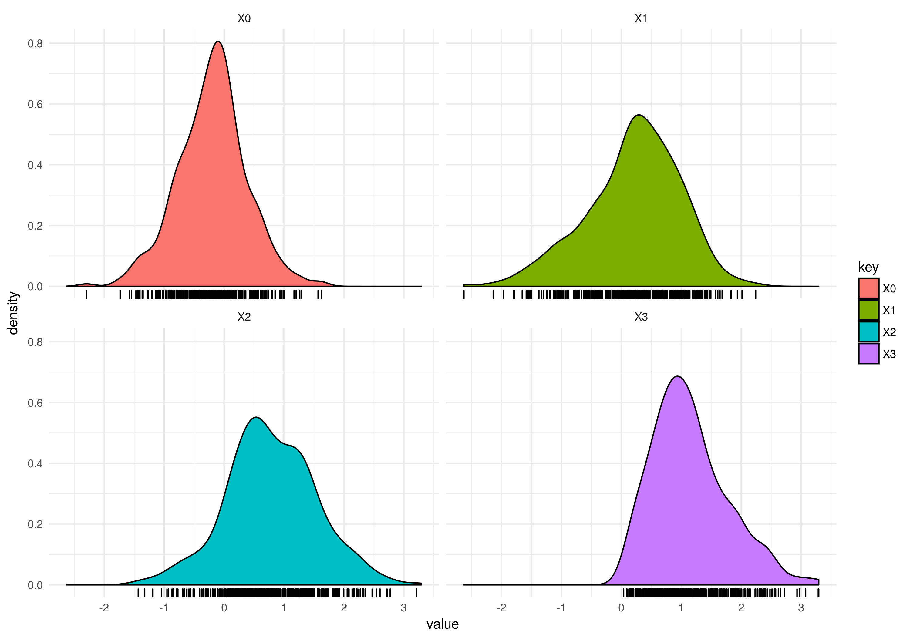
You can see that and should be around meanwhile and should be around . But several other solutions exist as illustrated. So naturally this uncertainty about what the parameters should exactly be could be taken into account by a learning agent.
Conclusion
We have implemented a reinforcement learning agent who acts in an environment with the purpose of maximizing the future reward. We have also discounted that future reward in the code but not covered it in the math. It’s straightforward though. The concept of being able to learn from your own mistakes is quite cool and represents a learning paradigm which is neither supervised nor unsupervised but rather a combination of both. Another appealing thing about this methodology is that it is very similar to how biological creatures learn from interacting with their environment. Today we solved the CartPole but the methodology can be used to attack far more interesting problems.
I hope you had fun reading this and learned something.
Happy inferencing!