There’s a new kid on the inference block called “Edward” who is full of potential and promises of merging probabilistic programming, computational graphs and inference! There’s also talk of a 35 times speed up compared to our good old reliable fellow “Stan”. Today I will run some comparisons for problems that currently interest me namely time series with structural hyperparameters.

To start things off and make sure we have all our ducks in a row for running edward we need to install it using the python installer called pip which is available in most linux distros. I will use pip3 here because I use python3 instead of python2. It shouldn’t matter which one you choose though. So go ahead and install “Edward”.

sudo pip3 install edward

If you ran this in the console you should now have a working version of Edward installed in your python environment. So far so good. Just to make sure it works we will run a small Bayesian Neural Network with Gaussian priors for the weights. This is the standard example from Edwards web page. It uses a Variational Inference approach to turn the sampling problem into an optimization problem by approximating the target posterior by a multivariate Gaussian. This approach works ok for quite a few problems. However, it is a tad hyped as a general purpose inference sampler and should not be considered as a replacement for a real sampler. In either case try to run the code below and check it out. For this toy dataset it works fine. ;)

from __future__ import absolute_import
from __future__ import division
from __future__ import print_function

import edward as ed
import numpy as np
import tensorflow as tf

from edward.models import Normal

def build_toy_dataset(N=50, noise_std=0.1):
  x = np.linspace(-3, 3, num=N)
  y = np.cos(x) + np.random.normal(0, noise_std, size=N)
  x = x.astype(np.float32).reshape((N, 1))
  y = y.astype(np.float32)
  return x, y

def neural_network(x, W_0, W_1, b_0, b_1):
  h = tf.tanh(tf.matmul(x, W_0) + b_0)
  h = tf.matmul(h, W_1) + b_1
  return tf.reshape(h, [-1])


ed.set_seed(42)

N = 50  # number of data ponts
D = 1   # number of features

# DATA
x_train, y_train = build_toy_dataset(N)

# MODEL
W_0 = Normal(mu=tf.zeros([D, 2]), sigma=tf.ones([D, 2]))
W_1 = Normal(mu=tf.zeros([2, 1]), sigma=tf.ones([2, 1]))
b_0 = Normal(mu=tf.zeros(2), sigma=tf.ones(2))
b_1 = Normal(mu=tf.zeros(1), sigma=tf.ones(1))

x = x_train
y = Normal(mu=neural_network(x, W_0, W_1, b_0, b_1),
           sigma=0.1 * tf.ones(N))

# INFERENCE
qW_0 = Normal(mu=tf.Variable(tf.random_normal([D, 2])),
              sigma=tf.nn.softplus(tf.Variable(tf.random_normal([D, 2]))))
qW_1 = Normal(mu=tf.Variable(tf.random_normal([2, 1])),
              sigma=tf.nn.softplus(tf.Variable(tf.random_normal([2, 1]))))
qb_0 = Normal(mu=tf.Variable(tf.random_normal([2])),
              sigma=tf.nn.softplus(tf.Variable(tf.random_normal([2]))))
qb_1 = Normal(mu=tf.Variable(tf.random_normal([1])),
              sigma=tf.nn.softplus(tf.Variable(tf.random_normal([1]))))

inference = ed.KLqp({W_0: qW_0, b_0: qb_0,
                     W_1: qW_1, b_1: qb_1}, data={y: y_train})


# Sample functions from variational model to visualize fits.
rs = np.random.RandomState(0)
inputs = np.linspace(-5, 5, num=400, dtype=np.float32)
x = tf.expand_dims(tf.constant(inputs), 1)
mus = []
for s in range(10):
  mus += [neural_network(x, qW_0.sample(), qW_1.sample(),
                         qb_0.sample(), qb_1.sample())]

mus = tf.stack(mus)

sess = ed.get_session()
init = tf.global_variables_initializer()
init.run()

import pandas as pd

# Prior samples
outputs = mus.eval()
mydf=pd.DataFrame(outputs)
mydf.to_csv("mydfprior.csv")

# Inference
inference.run(n_iter=500, n_samples=5)

# Posterior samples
outputs = mus.eval()
mydf=pd.DataFrame(outputs)
mydf.to_csv("mydfpost.csv")

Checking the priors

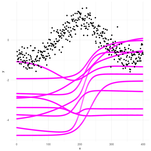
If you ran the code you will now have two files called mydfprior.csv and mydfpost.csv which contains, surprise, surprise, your prior and posterior curves based on the samples. As always we plot out the consequence of our priors and check what happens. In the plot below you can see that our priors for the Bayesian Neural Network do not really produce curves that resembles what we’re looking for. Not to worry my friends; we don’t actually need them to. Look through the graph and make sure you understand why the plot looks the way it does.

plot of chunk Prior plot

Checking the posteriors

The problem with the world is not that people know too little. It’s that they know so many things that just ain’t so. – Mark Twain

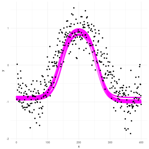
So the priors hopefully makes sense to you now. How about our posterior? Well as you can see below this plot makes a lot more sense compared to the data we’re trying to make sense of. However, you can clearly see some uncertainty in there as well. This is key, since no matter which model we choose there will always be elements of uncertainty involved. The great thing about science is that we don’t have to pretend to know everything. We’re perfectly comfortable admitting our ignorence. The probabilistic framework allows us to quantify that ignorance! If you think that sounds like a bad idea I suggest you take a look at the quote above.

plot of chunk Post plot

A more real world problem

A first look at the data

There are few real world problems as pressing as that of global warming. Whenever I’m talking about global warming I feel there are two responses I get which are basically binomially distributed in which the majority of people quickly gets it and the other part are oblivious to facts presented to them. In reality there can be little to no doubt that humans are causing the green house effect. The plot below shows the evolution of the temperature anomaly over time since the 1850’s until present time.

plot of chunk globwarmdata

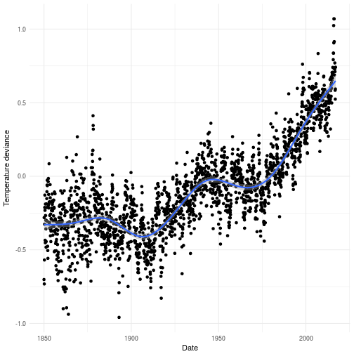
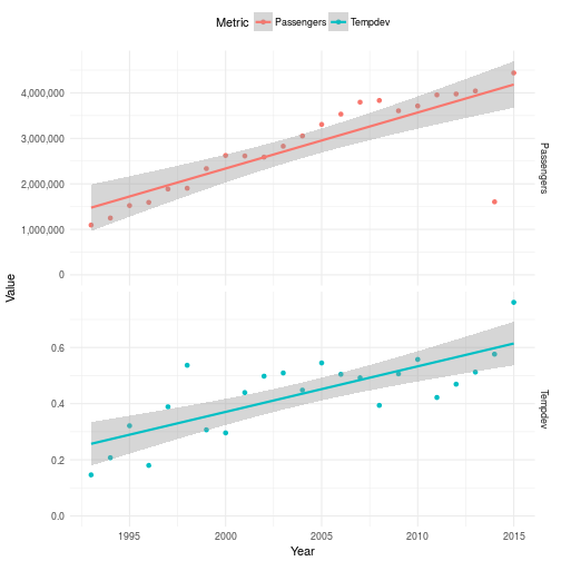
As you see there is a clear trend showing that the world is getting warmer. So global warming is indeed happening and it’s causing some very measurable real problems for us. There are lobbyist organizations around the world who wishes to tell you that this is not really caused by our increased CO2 emissions since they have well ulterior motives. If we plot the number of passenger per year in the same plot as the deviance of temperature it’s also quite apparent that something here might be at least weakly related. However, in order to really prove that we need more work than I’m going to do in this post. This post is about Edward and Error correction models and not Global warming.

plot of chunk jointplot

Specifying a model

As you might have noticed these data seem a bit like they are suffering from measurament errors. Especially the temperature but also the passengers. So when we also cannot trust the data to be point measurements what do we do? Well we create an error correction model. Since we are using probability we can express any kind of measurements as a probabilistic process. Below you’ll find code for the error correction model for the deviance in global temperature expressed in Edward. Mathematically the error correction model is

$\begin{align} X_t & \sim \mathcal N(\mu_{X,t}, \sigma_X)\\ \mu_{X,t} &\sim \mathcal N(0, 0.5)\\ \sigma_X &= 0.1 \end{align}$

where you can see that we fixed the noise so that we inform the model of the scale of the errors that we believe we will observe. If this is set too high then naturally nothing will emerge since the error is much larger than the signal. Be aware of these things in general when you express your likelihood functions!

Check out the math above and make sure you understand the code below to see how Edward materializes this model. It’s slightly different from Stan but you should be able to recognize most of the model setup. Do not worry too much about all the book keeping for extracting and merging the priors and posteriors. Especially the last part where I export the distributions. I do this because the plots I will show you soon will be done in R. Not because they cannot be done in Python, but because doing them in python makes me want to kill myself.

import tensorflow as tf
import edward as ed
import pandas as pd
import numpy as np
from ggplot import *
from edward.models import Normal, Bernoulli
import matplotlib.pyplot as plt

mydf = pd.read_csv("../humanglobwarm.csv")

N = mydf.shape[0]
D = mydf.shape[1]

# Define the model
x_mu = Normal(mu=tf.zeros(N), sigma=0.5*tf.ones([]))
x = Normal(mu=x_mu, sigma=0.1*tf.ones([]))

# VI placeholder
qx_mu = Normal(mu=tf.Variable(tf.zeros(N)), sigma=tf.nn.softplus(tf.Variable(0.5*tf.ones(N))))

# Set up data and the inference method to Kullback Leibler
x_train = mydf.get("Tempdev").reshape([N,1])
sess = ed.get_session()
data = {x: x_train[:,0]}
inference = ed.KLqp({x_mu: qx_mu}, data)

# Set up for samples from models
mus = []
for i in range(10):
    mus += [qx_mu.sample()]

mus = tf.stack(mus)

# Inference: More controlled way of inference running
inference.initialize(n_print=10, n_iter=600)
init = tf.global_variables_initializer()
init.run()

# Prior samples
outputs = mus.eval()
priordf=pd.DataFrame(outputs)
priordf['Sample']=["Sample"+str(x) for x in list(range(10))]
priordf=pd.melt(priordf, id_vars="Sample")
ggplot(priordf, aes(y="value", x="variable", color="Sample")) + geom_line()
priordf['Type']='Prior'

# Run Inference
for _ in range(inference.n_iter):
  info_dict = inference.update()
  inference.print_progress(info_dict)

inference.finalize()

# Posterior samples
outputs = mus.eval()
postdf=pd.DataFrame(outputs)
postdf['Sample']=["Sample"+str(x) for x in list(range(10))]
postdf=pd.melt(postdf, id_vars="Sample")
ggplot(postdf, aes(y="value", x="variable", color="Sample")) + geom_line()
postdf['Type']='Posterior'

# One glorious data frame for export
tmpdf = pd.concat([priordf, postdf])
tmpdf.to_csv("errorcorrsamplesdf.csv")

Did you get through the code? Good, then let’s have a look at our dear posteriors and priors and data! We will start off by looking at 10 samples from the priors and posteriors. The x-axis in the plot below represents the years 1993 to 2015 where 0 is 1993 and 2015 is 22.

plot of chunk errorcorrmodel

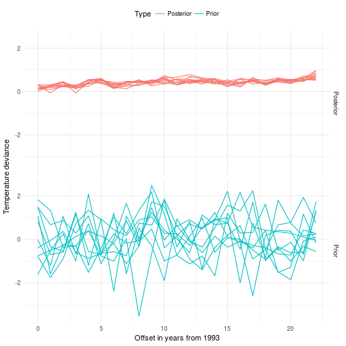
We may want to look into what the average effect of the error correction model is and compare it to the data we observed. As you can see here we extracted a new mean for every observed point. So it’s not surprising that it’s consistent with the data. However, do you have any observations regarding the uncertainty of the likelihood? I’m sure you do, so play around with it and check what happens. Remember that the sigma for the latent variable quantifies the uncertainty of the location of the mean but doesn’t state anything about what the likelihood will support.

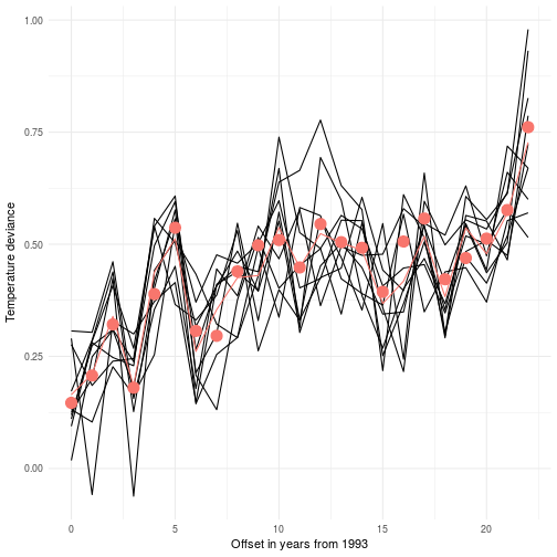
plot of chunk errorcorrmodelpostvsdata

Every data point in the graph above is marked with a red dot. The black lines are sampled from the posterior. These lines should be viewed as alternative realizations of the real unknown (latent) deviance in temperature. This construct allows us to not put undue confidence in the data we measured. In fact many data sources that are considered absolute are in fact inherently noisy.

Putting it in a regression formulation

We can of course formulate this as a regression problem where the likelihood is set up on the error correction itself. This means that if we get noisy measurements it’s the random variable that’s regressed. The benefit is that we don’t have to take the data at face value and neither does the model. Remember, uncertainty is not a bad thing as long as it can be quantified. Mathematically it looks like this

$\begin{align} X_t & \sim \mathcal N(\mu_{X,t}, \sigma_X)\\ \mu_{X,t} &\sim \mathcal N(\beta Z_t+\alpha, 0.5)\\ \beta & \sim \mathcal N(0, 1)\\ \alpha & \sim \mathcal N(0, 0.1)\\ \sigma_X &= 0.1 \end{align}$

where $X_t$ and $Z_t$ is the deviance in temperature and number of passengers transported by airplane at year $t$ respectively. The other variables quantify dynamics and uncertainty. The priors are specified quite widely to capture a broad spectrum of possibly consistent models. This model can also be sampled using Edward but I’ll leave that as an exercise for you to solve.

Conclusions from my simulations

So I played around with Edward and it took a bit of time to get used to the Edward way of doing things. Mainly because it’s so tightly connected to tensorflow. In general I like the idea of Edward and the flexibility in modeling that it allows for. That being said I think as of now the language is a bit young still. The Variational Inference approach (which is the only one I used in this post) works ok but when your priors are not in the vicinity of the final solution it rarely finds the correct posterior. There also seems to be quite heavy problems with varying scales of covariates. As such you should probably always work with normalized data when using Edward. To summarize the recommendations from this post

Always normalize your data when working with Edward
Make sure your priors are in the vicinity of the final solution, i.e., for simple models you can use a maximum likelihood estimate as a starting point
Never base your final inference on a variational algorithm; Instead always run a full sampler to verify and obtain the true posterior
Edward is cool and I will keep following it but for now I will stay with Stan for my probabilistic programming needs

Happy inferencing!