Confidence intervals are as beautiful as they are deceiving. They’re part of an elegant theory of mathematical statistics which has been abused since the dawn of time. Why do I say abused? Well quite frankly because literally everyone gets it wrong.. Now in order to subsantiate my claims let’s have a look at what the confidence interval really is mathematically by inspecting the following formula

$P_\theta\left(a(X)<\theta<b(X)\right)=\gamma,\, \forall \theta \in \mathbb{R}$

where $X$ is a random sample describing data generated by a process controlled by a fixed parameter $\theta$ . The $\gamma$ is the desired confidence level meanwhile the functions $a$ and $b$ are the lower and upper functions generating the boundary of the interval for a random sample. So what does this equation really say? Glad you asked, it states the following:

For a random sample of the data, the confidence interval as defined by the random variables $a$ and $b$ will contain the true value of the parameter $\theta$ with a probability of $\gamma$ .

An interesting thing about this interval is that it by design has to contain the unknown fixed parameter $\theta$ , no matter what that value might be, with a probability of $\gamma$ across all sampled data sets. It does NOT, however, say that the probability that the true value of $\theta$ for a realized data sample lies in the interval calculated for that very sample! Ok, fine! So then why do we state it probabalistically? The answer to this is also simple, because we are stating a probability distribution over random samples of $X$ controlled by the parameter $\theta$ . Once we have observed (sampled) a specific realization of that data the probability is gone. The only thing you can state after observing the data, in this setting, is

The realized interval at hand either contains the true value of the parameter or it does not.

That’s it folks, there is nothing more you can say about that. Thus, the conclusion here is that confidence intervals only speak about probabilities for repeated samples and measurements of the parameter of interest. In other words, the probability distribution is over the data and not the parameter.

Now don’t get me wrong, this is a really useful tool to have in your statistical toolbox and will for sure be helpful when you have access to multiple data sets measuring the same phenonemna. However, if you have just one realized data set, then a confidence interval is hardly what you want to express to yourself or others as a finding.

The remedy

Since we just loooked at the problems with the confidence interval you might wonder what we could do instead to quantify the uncertainty of our estimate given the data we currently do have. It turns out that we can use the same starting point as before but instead of viewing the data as random, we consider instead the parameter $\theta$ to be random and the data to be observed and fixed. This means that the interval now becomes

$P_\theta\left(a(x)<\Theta<b(x)\,\middle |\,X=x\right)=\gamma$

which expresses uncertainty in what we are actually interested in measuring. To not confuse it with the confidence interval I’ll use the $\Theta$ as the parameter of interest to highlight that it’s the focal point of the distribution. In addition I’ll call this the credibility interval instead. This is not my notation but widely used terminology. Now, we have a very natural way to relate the outcome to probability. We could for example set the degree of belief to 90\% and say the following:

The degree of my belief that the parameter is indeed in this interval is 90%.

As previously mentioned, this statement is reserved for credibility intervals and cannot, I reapeat, cannot be used in the setting of a confidence interval. Do not rest your minds until you understand this.

A simple polynomial regression example

If we take a look at a simple polynomial example we can illustrate some differences and similarities between the two approaches. In this scenario we have a noise model $y\sim\mathcal{N}\left(-2x^2+200x+1000, 30\sigma_x\right)$ which is depicted below for 100 samples. The blue dots are the measured noisy samples, while the red dots are the “truth”.

plot of chunk datablock

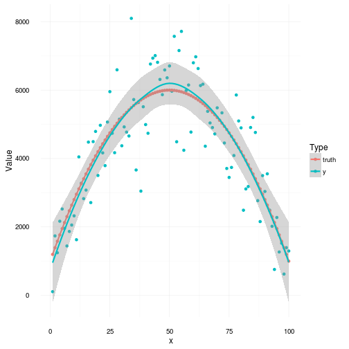
The question now is how a normal linear regression and a bayesian linear regression, with uninformative priors, handle this and what the inference about the sought parameters might be. Let’s start by looking at what our linear regression model finds in comparison to the Bayesian approach.

Parameter	Freq	Bayes
Intercept	959.19 (382.23, 1536.15)	940.97 (297.82, 1511.04)
X	197.41 (171.04, 223.78)	197.18 (174.18, 229.97)
X²	-1.98 (-2.24, -1.73)	-1.97 (-2.29, -1.75)

Well hang on a moment, these results are as far as I can see more or less identical! Indeed you are right, as you might recall I did say that we were doing a non-informative Bayes linear regression which means that all of our parameters were fed with uniform non-informative priors. It’s rather obvious that there’s really no qualitative difference between the confidence intervals created by the frequentist approach and the credibility intervals created by the Bayesian approach. Does this mean that they are the same? Well, no. They are the same because in our first attempt at being Bayesian we assumed flat uniform priors which means that we provided purely non-informative priors. As such the Bayesian approach is purely data driven which means that the likelihood determines everything. This illustrates nicely the point that maximum likelihood for a linear model is just a special case of the fully Bayeian model with uniform priors.

If we investigate one of the parameters more closely we can see that the intercept term is way off. It should be 1000 but is much lower in the estimates. The reason for this is the random noise that was added of course. But even so, couldn’t we do better? Yes we can. We can look at the data and see that it looks like it’s peaking at x=50 so let’s put a prior on our parameters reflecting that belief. The new results for Bayes2 is given below.

Parameter	Freq	Bayes 2
Intercept	959.19 (382.23, 1536.15)	941.32 (468.09, 1320.55)
X	197.41 (171.04, 223.78)	197.55 (177.34, 224.57)
X²	-1.98 (-2.24, -1.73)	-1.98 (-2.25, -1.77)

Now it’s quite apparent to see that we are in much better shape regarding the intercept term while the other estimates stayed more or less in the same range. They were also never bad to begin with.

Repeated measurements

Let’s see what happens if we repeat the analysis 100 times. In this scenario we have 100 researchers with 100 realized data sets from the same underlying process. How will their inferences look?

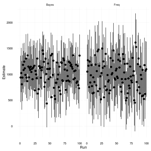
plot of chunk confidencebayesandfreq1

The uncertainty, of the confidence interval for the freqeuntist approach and of the parameter estimate in the Bays 2 model are rather different. The prior we added to the Bayes model obviously helps us in making educated inferences about the true parameter value. The variation of the estimated parameter is 21 per cent lower for the Bayes 2 model compared to the frequentist approach. Further the average difference between the upper and lower limits is 21 per cent lower for the Bayes 2 model.

Summary

So let’s round this up by stating that confidence intervals are useful nifty little things that are exceedingly open to misinterpretation. Use them if you want to but make sure you understand them. The following little list is useful to remember.

A confidence interval does not say anything about the probability of the sought parameter to be inside a specific interval
A confidence interval is a probability distribution over the data generated by a fixed parameter and not over the parameter
Once a confidence interval has been realized (measured) by observing data it is no longer a probability; it either contains the parameter value sought or it does not