Have you ever thought about how strong a prior is compared to observed data? It’s not an entirely easy thing to conceptualize. In order to alleviate this trouble I will take you through some simulation exercises. These are meant as a fruit for thought and not necessarily a recommendation. However, many of the considerations we will run through will be directly applicable to your everyday life of applying Bayesian methods to your specific domain. We will start out by creating some data generated from a known process. The process is the following.

$y_t=\sin\left(\frac{x_t}{10}\right)+\cos(z_t)+5d_t+4+\epsilon_t$

It features a cyclic process with one event represented by the variable $d$ . There is only 1 observation of that event so it means that maximum likelihood will always assign everything to this variable that cannot be explained by other data. This is not always wanted but that’s just life. The data and the maximum likelihood fit looks like below.

plot of chunk lmfit

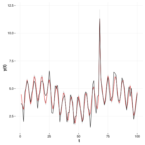
The first thing you can notice is that the maximum likelihood overfits the parameter in front of $d$ by 20.2 per cent since the true value is 5.

	Estimate	Std. Error	t value
(Intercept)	4.03	0.05	78.97
sin(x/10)	0.97	0.07	13.25
cos(z)	1.20	0.07	17.14
d	6.01	0.50	12.12

Now imagine that we do this the Bayesian way and fit the parameters of the generating process but not the functional form. As such we will sample the beta parameters with no priors what so ever and look at what comes out. In the plot below you will see the truth which is $y$ and 3 lines corresponding to 3 independent samples from the fitted resulting posterior distribution.

plot of chunk test

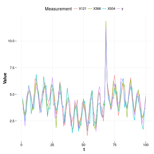
Pretty similar to the maximum likelihood example except that now we also know the credibility intervals and all other goodies that the Bayesian approach gives us. We can summarize this quickly for the beta parameters. So we can see that we are still overfitting even though we have a Bayesian approach.

parameter	Q1	mean	Q3
beta_d	5.69	6.03	6.33
beta_x	0.93	0.98	1.03
beta_z	1.14	1.19	1.23

Now to the topic at hand! How strong are priors compared to data?

About weak priors and being ignorant

In order to analyze the strength of priors we will consistently set ever more restrictive priors and see what happens to the result. Remember that the happy situation is that we know the truth. We will start by building a model like shown below which means that we will only assign priors to the betas and not the intercept.

$\begin{align} y_t &\sim N(\mu_t, \sigma)\\ \mu_t &=\beta_x \sin(x_t/10) + \beta_z \cos(z_t) + \beta_d d_t + \alpha\\ \beta_x &\sim N(0, 1000)\\ \beta_z &\sim N(0, 1000)\\ \beta_d &\sim N(0, 1000)\\ \alpha &\sim U(-\inf, \inf)\\ \sigma &\sim U(0.01, \inf) \end{align}$

Thus this model conforms to the the same process as before but with weak priors introduced. The priors here state that the $\beta$ parameters are all Gaussian distributions with a lot of variance around them meaning that we are not very confident about what these values should be. If you look at the table above where we had no priors, which basically just means that our priors were uniform distributions between minus infinity and infinity, you can see that the inference is not much different at all.

parameter	Q1	mean	Q3
beta_d	5.69	6.01	6.34
beta_x	0.93	0.98	1.02
beta_z	1.15	1.20	1.24

One thing to note is that the credible interval has not shrunken which means that the models uncertainty about each parameters is about the same. Now why is that? Well for starters in the first model we even if we “believed” that infinity was a reasonable guess for each parameter the sampler found it’s way. The mean of the posterior distributions for each parameter is nearly identical between the models. So that’s great. Two infinitely different priors results in the same average inference. Let’s try to see at what scale the priors would change the average inference. See the new model description here.

$\begin{align} y_t &\sim N(\mu_t, \sigma)\\ \mu_t &=\beta_x \sin(x_t/10) + \beta_z \cos(z_t) + \beta_d d_t + \alpha\\ \beta_x &\sim N(0, 10)\\ \beta_z &\sim N(0, 10)\\ \beta_d &\sim N(0, 10)\\ \alpha &\sim U(-\inf, \inf)\\ \sigma &\sim U(0.01, \inf) \end{align}$

Now what does that look like for our inference? It looks like this!

parameter	Q1	mean	Q3
beta_d	5.70	6.01	6.34
beta_x	0.93	0.98	1.03
beta_z	1.16	1.20	1.24

Still not a lot of difference so let’s do a scale of 10 reduction again.

$\begin{align} y_t &\sim N(\mu_t, \sigma)\\ \mu_t &=\beta_x \sin(x_t/10) + \beta_z \cos(z_t) + \beta_d d_t + \alpha\\ \beta_x &\sim N(0, 1)\\ \beta_z &\sim N(0, 1)\\ \beta_d &\sim N(0, 1)\\ \alpha &\sim U(-\inf, \inf)\\ \sigma &\sim U(0.01, \inf) \end{align}$

Here we can totally see a difference. Look at the mean for parameter $\beta_d$ in the table below. It goes from 6.03 to 4.73 which is a change of 21 per cent. Now this average is only 5.4 per cent different from the truth.

parameter	Q1	mean	Q3
beta_d	4.40	4.73	5.07
beta_x	0.93	0.98	1.03
beta_z	1.16	1.20	1.25

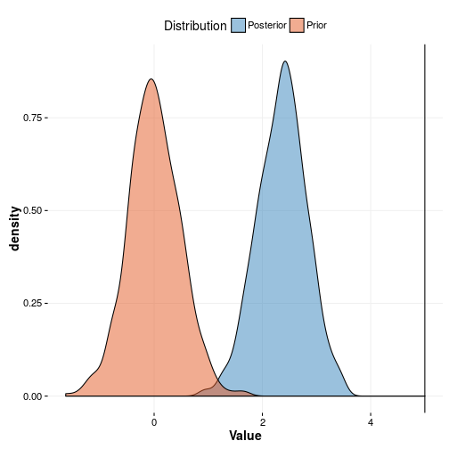
But let’s take a while to think about this. Why did this happen? The reason is that your knowledge can be substantial. Sometimes a lot more substantial than data. So your experience about this domain SHOULD be taken into account and weighted against the evidence. Now it is up to you to mathematically state your experience which is what we did in the last model. Before you start to argue with my reasoning take a look at the plots where we plot the last prior vs the posterior and the point estimate from our generating process.

plot of chunk priorpostplot

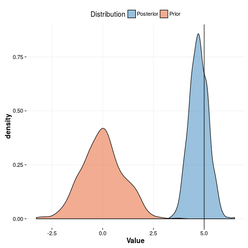
As you can see the prior is in the vicinity of the true value but not really covering it. This is not necessarily a bad thing as being ignorant allows data to move you into insane directions. An example of this is shown in the plot below where we plot the prior from model three against the posterior of model three. It’s apparent that the data was allowed to drive the value to a too high value meaning that we are overfitting. This is exactly why maximum likelihood suffers from the curse of dimensionality. We shouldn’t be surprised by this since we literally told the model that a value up to 10 is quite probable.

plot of chunk priorpostplot2

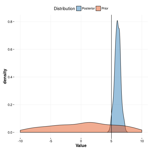
We can formulate a learning from this.

The weaker your priors are the more you are simulating a maximum likelihood solution.

About strong priors and being overly confident

If the last chapter was about stating your mind and being confident in your knowledge about the domain there is also a danger in overstating this and being overly confident. To illustrate this let’s do a small example where we say that the beta’s swing around 0 with a standard deviation of $0.5$ which is half the width of the previous. Take a look at the parameter estimates now.

$\begin{align} y_t &\sim N(\mu_t, \sigma)\\ \mu_t &=\beta_x \sin(x_t/10) + \beta_z \cos(z_t) + \beta_d d_t + \alpha\\ \beta_x &\sim N(0, 0.5)\\ \beta_z &\sim N(0, 0.5)\\ \beta_d &\sim N(0, 0.5)\\ \alpha &\sim U(-\inf, \inf)\\ \sigma &\sim U(0.01, \inf) \end{align}$

parameter	Q1	mean	Q3
beta_d	2.05	2.36	2.66
beta_x	0.90	0.96	1.02
beta_z	1.16	1.21	1.27

It’s quite apparent that here we were overly confident and the results are now quite a bit off from the truth. However, I would argue that this is a rather sane prior still. Why? Because we had no relation to the problem at hand and it’s better in this setting to be a bit conservative. As such we were successful. We stated our mind and the “one” data point updated it by a lot. Now imagine if we would have had two? As such maybe it’s not so bad that one data point was able to update our opinion quite a bit and maybe it wasn’t such a bad idea to be conservative in the first place?

plot of chunk priorpostplot3

Naturally whether or not it’s recommended to be conservative is of course up to the application at hand. For an application determining whether a suspect is indeed guilty of the crime in the face of evidence it is perhaps quite natural to be skeptic of the “evidence” meanwhile for a potential investment it may pay off to be more risky and accept a higher error rate at the hope of a big win.

Conclusion

So what did we learn from all of this? Well hopefully you learned that setting priors is not something you learn over-night. It takes practice to get a feel for it. However, the principles are exceedingly obvious. I will leave you with some hard core advice on how to set priors.

Always set the priors in the vicinity of what you believe the truth is
Always set the priors such that they reflect the same order of magnitude as the phenomenon you’re trying to predict
Don’t be overconfident, leave space for doubt
Never use completely uninformative priors
Whenever possible refrain from using uniform distributions
Always sum up the consequence of all of your priors such that if no data was available your model still predicts in the same order of magnitude as your observed response
Be careful, and be honest! Never postulate very informative priors on results you WANT to be true. It’s OK if you BELIEVE them to be true. Don’t rest your mind until you see the difference.

Happy hacking!